
Numpy內容
Numpy是Python中用於科學計算的核心庫,提供高性能的多維數組對象(ndarray)及運算工具。其核心功能包括數組創建、數學運算、線性代數、隨機數生成等。實戰中常用於數據處理、數值模擬和矩陣運算。
1. Numpy的數組對象ndarray
ndarray 是 Numpy 的核心數據結構,支持多維數組操作。其特點包括高效存儲、廣播機制和豐富的數學運算接口。
1. 1python和ndarray數組運算的比較
import numpy as np

def pySum():
    a = [1, 2, 3]
    b = [2, 3, 4]
    c = []
    for i in range(len(a)):
        c.append(a[i] ** 2 + b[i])
    return c

print(pySum())

# 1.2 ndarray
def npSum():
    a = np.array([1, 2, 3])
    b = np.array([2, 3, 4])
    c = a ** 2 + b
    return c

print(npSum())
1. 2 ndarray方法
ndarray 方法概述
NumPy 的 ndarray(N-dimensional array)是多維數組的核心數據結構,支持高效數值運算和批量操作。
創建與初始化
np.array(): 從列表或元組創建數組
arr = np.array([1, 2, 3]) # 一維數組np.zeros()/np.ones(): 生成全 0 或全 1 數組
arr = np.zeros((2, 3)) # 2行3列的零矩陣np.arange(): 生成等差序列
arr = np.arange(0, 10, 2) # [0, 2, 4, 6, 8]常用的方法
import numpy as np
def ndMethods():
    a = np.array([[1, 2, 3],
                 [4, 5, 6]])

    print("ndim(維度的個數):{}".format(a.ndim))
    print("shape(幾行幾列):{}".format(a.shape))
    print("size(元素的個數):{}".format(a.size))
    print("dtype(元素的類型):{}".format(a.dtype))
    print("itemsize(每個元素的大小,字節為單位):{}".format(a.itemsize))
ndMethods()
2. 數據的CSDV文件
CSV(Comma-Separated Values,逗號分隔值,有時也稱為字符分隔值,因為分隔字符也可以不是逗號)
其文件以純文本形式存儲表格數據(數字和文本)。
scv侷限性:只能讀取和存儲一維數組和二維數組
多維數組的讀取:a.tofile(frame, sep="", format="%s") --- 寫入文件(不指定類型時候,是純文本)
np.fromfile(frame, dtype=float, count=-1, sep="") --- -1表示讀入整個文件(可修改讀入部分文件)
Numpy的便捷文件存取:
np.save(frame, array)或np.savez(frame, array) --- frame文件名稱,以.npy為擴展名,壓縮擴展名為.npz,後者壓縮格式存儲文件中
np.load(frame)
import numpy as np
# 寫CSV文件np.savetxt
def CsvWriter():
    a = np.arange(100).reshape(5, 20)
    print("原數據:\n{}".format(a))
    np.savetxt("a.csv", a, fmt="%.1f", delimiter=",")


CsvWriter()
# 讀CSV文件np.loadtxt
def CsvRead():
    b = np.loadtxt("a.csv", delimiter=",")
    print(b)


CsvRead()

# np.tofile()
def tofile_from():
    d = np.arange(100).reshape(5, 2, 10)
    print("原數據:\n{}".format(d))
    d.tofile("d.tofile", sep=",", format="%d")
    d.tofile("d.TofileNosep", format="%d")
    e = np.fromfile("d.tofile", dtype=int, count=-1, sep=",").reshape(2, 5, 10)
    print("讀取sep非空數據:\n{}".format(e))
    print("讀取sep為空數據:\n{}".format(np.fromfile("d.TofileNosep", dtype=int, count=-1, sep="").reshape(2, 10, 5)))
tofile_from()

f = np.random.randint(0, 50, (2, 3, 4))
np.save("f.save", f)
print(np.load("f.save.npy"))
np.savez("f.savez", f)
print("load_savez:\n{}".format(np.load("f.savez.npz")))
3. 函數介紹
3.1 Random隨機函數
NumPy的random子庫
使用方法:np.random.函數名
常見的函數:
rand(d0,d1,...,dn) --- 根據d0-dn創建隨機數數組,浮點數,[0, 1),均勻分佈
randn(d0,d1,...,dn) --- 根據d0-dn創建隨機數數組,標準正態分佈
randint(low,high,shape) --- 根據shape創建隨機整數或整數數組,範圍是[low,high)
seed(s) --- 隨機種子,s是給定的種子值,可使隨機生成的數組元素一樣
shuffle(a) --- 改變原數組,改變每一維相同列的元素順序
permutation(a) --- 不改變原數組,改變每一維相同列的元素順序
choice(a[,size,replace,p]) --- 一維數組a中以概率p抽取元素,形成大小為size的新數組,replace表示是否重複抽取(默認False)
隨機數函數:
uniform(low,high,size) --- 產生元素均勻分佈
normal(loc,scale,size) --- 產生元素正態分佈,loc均值,scale標準差
poisson(lam,size) --- 產生元素泊松分佈,lam隨機事件發生概率
import numpy as np
import random

a = np.random.rand(2, 4, 5)
print("rand:\n{}".format(a))
b = np.random.randn(2, 4, 5)
print("randn:\n{}".format(b))
np.random.seed(10)
c = np.random.randint(100, 200, (2, 4, 5))
print("randint:\n{}".format(c))
np.random.seed(10)
c = np.random.randint(100, 200, (2, 4, 5))
print("randint:\n{}".format(c))

print("---------------------------------------")
d = np.random.randint(100, 200, (3, 4))
print(d)
np.random.shuffle(d)
print(d)
e = np.random.randint(10, 100, (8,))
print(e)
print(np.random.choice(e, (3, 2), replace=False))
print(np.random.choice(e, (3, 2), p=e/np.sum(e)))

print("-------隨機生成函數3--------")
print(np.random.uniform(0, 10, (2, 3, 4)))
運行結果:
rand:
[[[0.79187961 0.35106545 0.83741265 0.07060377 0.57897558]
  [0.24786072 0.61053155 0.96720812 0.37647052 0.91915721]
  [0.23508372 0.59556412 0.98136907 0.19820676 0.72074763]
  [0.61126781 0.09021824 0.10949093 0.09702187 0.8664463 ]]

 [[0.25035799 0.4986956  0.16036751 0.69703055 0.21096326]
  [0.68698481 0.21196962 0.54689814 0.17170921 0.14839063]
  [0.68040513 0.65096094 0.42280268 0.87129442 0.08193161]
  [0.23646628 0.52076326 0.07578166 0.67691283 0.6124782 ]]]
randn:
[[[-0.97301268 -1.22476676 -0.25521379  1.51069476 -0.07100173]
  [ 0.92989698 -1.41605585  1.67700425 -0.26960737  0.25834075]
  [-0.18674952  0.89196952 -0.50971001  1.77603492  0.13947927]
  [-1.16224637 -0.43302191 -0.2248452  -0.36800825  0.85904455]]

 [[-1.23953705  0.69017062 -0.3968869  -1.18665731 -0.28199817]
  [-1.07569227 -0.53885996  0.15076961 -0.24731411 -0.5327221 ]
  [ 1.19748074 -0.54810851  0.81737705  2.48954932  1.18785129]
  [ 0.28493005  0.02141978 -1.25092627 -0.09025078  0.16962707]]]
randint:
[[[109 115 164 128 189]
  [193 129 108 173 100]
  [140 136 116 111 154]
  [188 162 133 172 178]]

 [[149 151 154 177 169]
  [113 125 113 192 186]
  [130 130 189 112 165]
  [131 157 136 127 118]]]
randint:
[[[109 115 164 128 189]
  [193 129 108 173 100]
  [140 136 116 111 154]
  [188 162 133 172 178]]

 [[149 151 154 177 169]
  [113 125 113 192 186]
  [130 130 189 112 165]
  [131 157 136 127 118]]]
---------------------------------------
[[193 177 122 123]
 [194 111 128 174]
 [188 109 115 118]]
[[194 111 128 174]
 [188 109 115 118]
 [193 177 122 123]]
[81 98 21 27 56 17 85 38]
[[17 38]
 [27 85]
 [81 21]]
[[85 98]
 [56 85]
 [38 21]]
-------隨機生成函數3--------
[[[8.75744495 2.96068699 1.31291053 8.42817933]
  [6.59036304 5.95439605 4.36353698 3.56250327]
  [5.87130925 1.49471337 1.71238598 3.97164523]]

 [[6.37951564 3.72519952 0.02406761 5.48816356]
  [1.26971841 0.79792681 2.35038596 6.59964947]
  [2.14953192 2.03046616 3.82865111 2.24872802]]]
3.2 統計函數
調用方法:np.函數名
常見函數:
sum()
mean()
average()
std()
var()
3.3 梯度函數
梯度:連續值之間的變化率,即斜率
常見的函數:
np.gradient(f) --- 計算數組f中元素的梯度,當f為多維時,計算每個維度的梯度
例如元素a的梯度計算 = (a下一個值 - a上一個值)/
如果a在一側:a在左側 = (a下一個值 - a)/1
a在右側 = (a - a的上一個值)/1
生成兩個梯度情況:行梯度,列梯度
import numpy as np
a = np.random.randint(0, 50, (3, 5))
print("原數組a:\n{}".format(a))
print("梯度:\n{}”".format(np.gradient(a)))
運行結果:
原數組a:
[[ 9  2  5 16 44]
 [ 5 46  6  5 39]
 [28 17 47 14 22]]
梯度:
(array([[ -4. ,  44. ,   1. , -11. ,  -5. ],
       [  9.5,   7.5,  21. ,  -1. , -11. ],
       [ 23. , -29. ,  41. ,   9. , -17. ]]), array([[ -7. ,  -2. ,   7. ,  19.5,  28. ],
       [ 41. ,   0.5, -20.5,  16.5,  34. ],
       [-11. ,   9.5,  -1.5, -12.5,   8. ]]))”

進程已結束,退出代碼0
4. 圖像的數組
fromarray() --- 實現array到image轉換
convert("L") --- 圖像轉換成灰度圖像(RGB圖像矩陣元素變成灰度值表示)
4.1 實例
from PIL import Image
import numpy as np
"""
    1. 圖片RGB格式
"""
im = np.array(Image.open("../image/P1_row.jpg"))
print(im.shape, im.dtype)  # (246, 320, 3) uint8

b = [255, 255, 255] - im
im = Image.fromarray(b.astype("uint8"))
im.save("../image/P2_row.jpg")

"""
    2. 圖片灰度格式
"""
im2 = np.array(Image.open("../image/P1_row.jpg").convert('L'))
print(im2.shape, im2.dtype)

c = 255 - im2
im22 = Image.fromarray(c.astype('uint8'))
im22.save("../image/P2_row(2).jpg")

# 區間變換
c = (100/255) * im2 + 150  # 區間變換
im22 = Image.fromarray(c.astype('uint8'))
im22.save("../image/P2_row(3).jpg")

# 像素平方
c = 255*(im2/255)**2  # 像素平方
im22 = Image.fromarray(c.astype('uint8'))
im22.save("../image/P2_row(4).jpg")

"""
    3. 圖像的手繪效果
            特徵:(1)黑白灰度
                 (2)邊界線條較重
                 (3)相同或相近色彩趨近白色
                 (4)略有光源效果
        手繪風格是在對圖像的進行灰度的基礎上由立體效果和明暗效果疊加生成的
            灰度代表圖像的明暗變化,梯度值表示灰度的變化率
                所以可通過調整梯度值,來間接改變圖像的明暗程度
            立體效果通過添加虛擬深度值來實現
"""
image = np.array(Image.open("../image/P1_row.jpg").convert('L')).astype('float')

depth = 10  # 範圍是(0-100)
grad = np.gradient(image)   # 取灰度值的梯度值
grad_x, grad_y = grad   # 分別取x、y軸的梯度值
grad_x = grad_x * depth / 100
grad_y = grad_y * depth / 100
A = np.sqrt(grad_x**2 + grad_y**2 +1.)
uni_x = grad_x / A
uni_y = grad_y / A
uni_z = 1. / A

vec_el = np.pi / 2.2  # 光源的俯視角度,弧度值
vel_ez = np.pi / 4.  # 光源的方位角度,弧度值
dx = np.cos(vec_el) * np.cos(vel_ez)  # 光源對x軸的影響
dy = np.cos(vec_el) * np.sin(vel_ez)  # 光源對y軸的影響
dz = np.sin(vec_el)

b = 255 * (dx * uni_x + dy * uni_y + dz * uni_z)  # 光源歸一化
b = b.clip(0, 255)

image = Image.fromarray(b.astype('uint8'))
image.save("../image/P2_row(5).jpg")
Matplotlib內容
Matplotlib是Python的2D繪圖庫,支持折線圖、散點圖、柱狀圖等可視化類型。通過pyplot模塊可快速生成圖表,適合數據分析和結果展示。
簡單介紹plt,以及相應的函數介紹
matplotlib.pyplot:是繪製各類可視化圖形的命令子庫,相當於快捷方式
1. 簡單繪製一個圖形
import matplotlib.pyplot as plt
import numpy as np

"""
    1. 簡單繪製一個圖形:
        savefig():將輸出的圖形存儲為文件,默認為PNG格式,可通過dpi修改輸出質量
                  dpi:每一英寸的空間中包含點的數量
        axis([a, b, c, d]):空值橫縱座標尺寸,橫軸[a,b];縱軸[c,d]
        subplot(nrows,ncols,plot_number):在全局繪圖區域中創建一個分區體系,並定位到一個子繪圖區域
                  表示nrows行,ncols列,當前在第plot_number區域中繪製
"""
plt.subplot(3, 2, 4)
plt.plot([0, 2, 4, 6, 8], [1, 1, 3, 5, 5])  # plot作用是將一組數據點連接起來
plt.ylabel("grad")
plt.axis([-1, 10, 0, 6])
plt.savefig("../img_plt/P1", dpi=600)
plt.show()
運行結果:

實例:
import matplotlib.pyplot as plt
import numpy as np
"""
2. 實例
"""
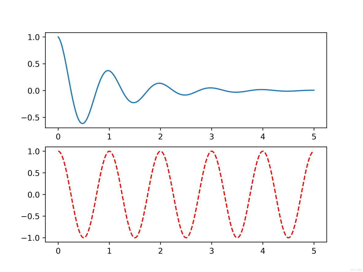
def f(t):
return np.exp(-t) * np.cos(2*np.pi*t)
plt.subplot(2, 1, 1)
a = np.arange(0.0, 5, 0.002)
plt.plot(a, f(a))
plt.subplot(2, 1, 2)
plt.plot(a, np.cos(2*np.pi*a), 'r--')
plt.savefig("../img_plt/P1_(2)", dpi=500)
plt.show()運行結果:
2. plot()函數
import numpy as np
import matplotlib.pyplot as plt
"""
plot函數參數介紹:
plt.plot(x,y,format_string,**kwargs)
format_string:控制曲線的格式字符串,可選
由顏色字符、風格字符和標記字符組成
可分開寫:1.color='green' --- 控制顏色
2.linestyle='dashed' --- 線條風格
3.marker='o' --- 標記風格
4.maekerfacecolor='blue' --- 標記的顏色
5.markersize=20 --- 標記大小
"""
"""
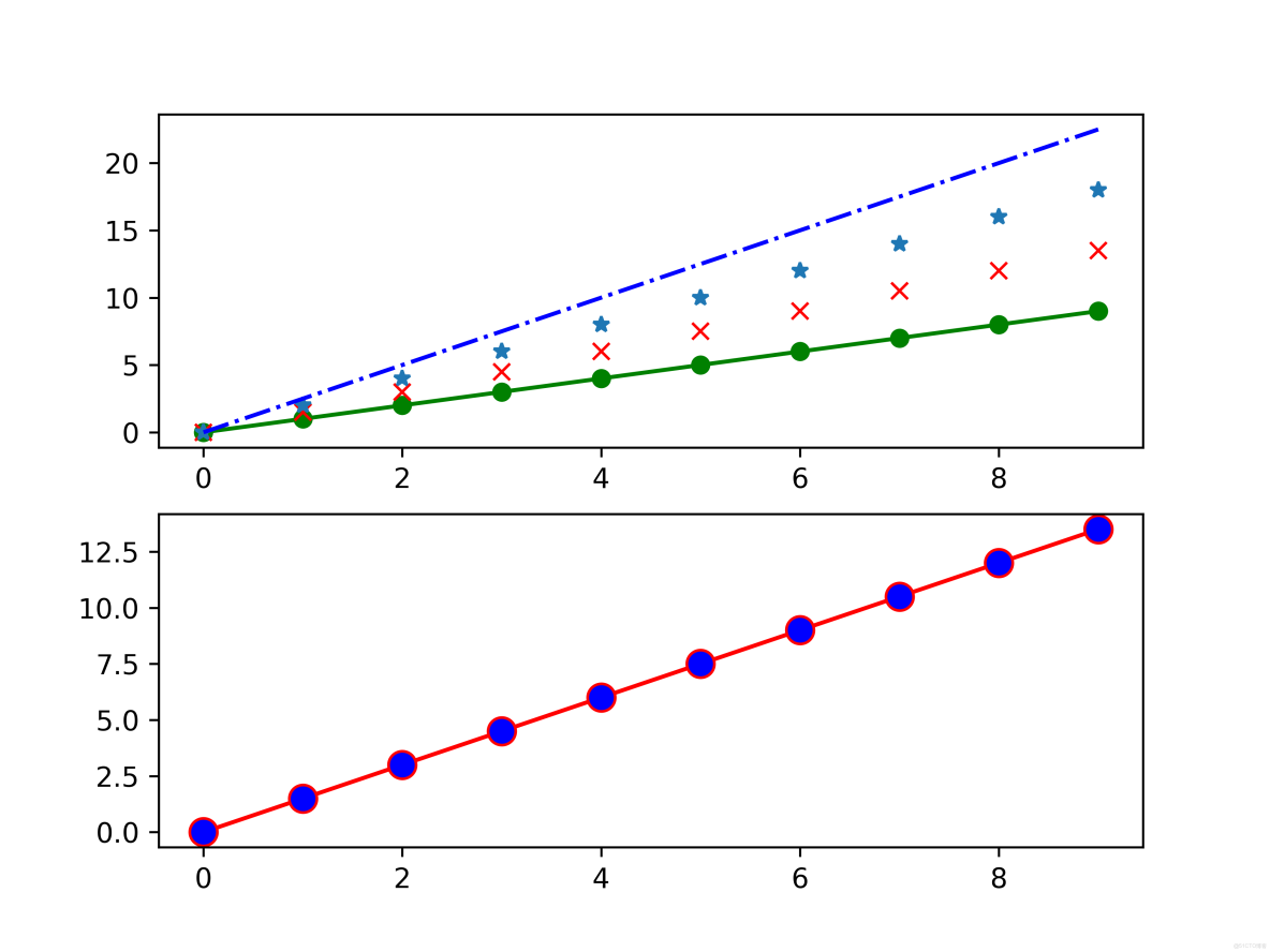
1. 繪製多條曲線
"""
plt.subplot(2, 1, 1)
a = np.arange(10)
plt.plot(a, a, 'go-', a, a * 1.5, 'rx', a, a * 2, '*', a, a * 2.5, 'b-.')
plt.subplot(2, 1, 2)
plt.plot(a, a * 1.5, color='r', linestyle='-', marker='o', markerfacecolor='b', markersize=10)
plt.savefig("../img_plt/P2_(1)", dpi=600)
plt.show()運行結果:
3. pyplot中文顯示
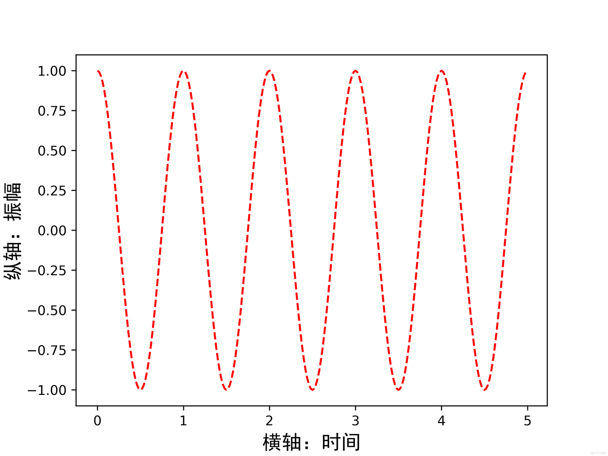
第一種方法:改變全局字體
pyplot並不默認支持中文顯示,需要reParams修改字體實現
reParams(font.family, font.style, font.size)
* 顯示字體的名字
* 字體風格,正常:normal;斜體:italic
* 字體的大小
import numpy as np
import matplotlib.pyplot as plt
import matplotlib

matplotlib.rcParams['font.family'] = 'STSong'
matplotlib.rcParams['font.style'] = 'italic'
a = np.arange(0.0, 5, 0.02)

plt.xlabel('橫軸:時間')
plt.ylabel('縱軸:振幅')
plt.plot(a, np.cos(2*np.pi*a), 'r--')
plt.show()
運行結果:
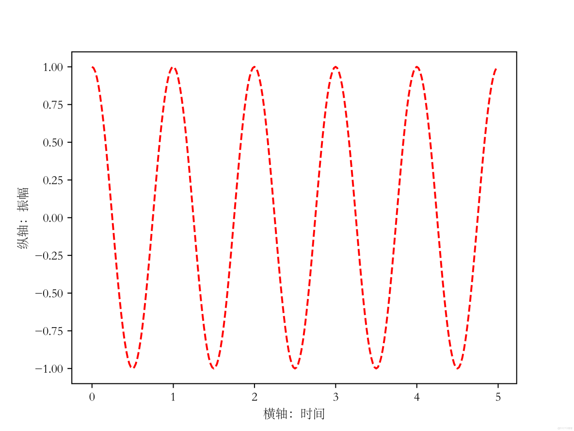
第二種方法:
在有中文輸入的地方,增加一個屬性:fontproperties
import numpy as np
import matplotlib.pyplot as plt

a = np.arange(0.0, 5, 0.02)

plt.xlabel('橫軸:時間', fontproperties='SimHei', fontsize=15)
plt.ylabel('縱軸:振幅', fontproperties='SimHei', fontsize=15)
plt.plot(a, np.cos(2*np.pi*a), 'r--')
plt.savefig("../img_plt/P3_(2)", dpi=600)
plt.show()
運行結果:
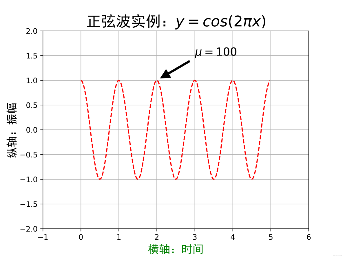
4. pyplot文本顯示
pyplot的文本顯示函數:
plt.xlabel()
plt.ylabel()
plt.title():對圖像整體增加文本標籤
plt.text():對任意位置增加文本,前兩位代表座標值
plt.annotate(s, xy=arrow_crd, xytext=text_crd, arrowprops=dict):在圖形中增加帶箭頭的註釋
s:註釋的字符串內容
xy:箭頭所在的位置
xytext:文本顯示的位置
arrowprops:字典類型,定義箭頭顯示的屬性
plt.grid(True):顯示網格
import matplotlib.pyplot as plt
import numpy as np
"""
    pyplot的文本顯示函數:
        plt.xlabel()
        plt.ylabel()
        plt.title():對圖像整體增加文本標籤
        plt.text():對任意位置增加文本,前兩位代表座標值
        plt.annotate(s, xy=arrow_crd, xytext=text_crd, arrowprops=dict):在圖形中增加帶箭頭的註釋
            s:註釋的字符串內容
            xy:箭頭所在的位置
            xytext:文本顯示的位置
            arrowprops:字典類型,定義箭頭顯示的屬性
        plt.grid(True):顯示網格
"""
plt.subplot(1, 1, 1)
a = np.arange(0.0, 5, 0.02)
plt.plot(a, np.cos(a * np.pi * 2), 'r--')
plt.xlabel('橫軸:時間', fontproperties='SimHei', fontsize=15, color='green')
plt.ylabel('縱軸:振幅', fontproperties='SimHei', fontsize=15)
plt.title('正弦波實例:$y=cos(2\pi x)$', fontproperties='SimHei', fontsize=20)
# plt.text(2, 1, r'$\mu=100$', fontsize=15)
plt.annotate(r'$\mu=100$', xy=(2, 1), xytext=(3, 1.5), arrowprops=dict(facecolor='black', shrink=0.1, width=2), fontsize=15)
plt.axis([-1, 6, -2, 2])
plt.grid(True)
plt.savefig("../img_plt/P4_(1)", dpi=600)
plt.show()
運行結果:
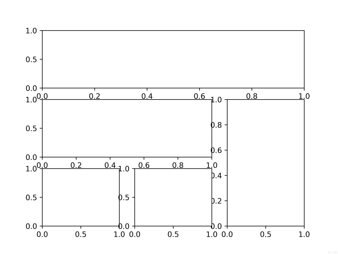
5. pyplot子繪圖區域
子區域隨意分區:
方法一:.subplot2grid()方法
plt.subplot2grid(GridSpec, CurSpec, colspan=1, rowspan=1)
理念:設定網格,選定網格,確定選中行列區域的數量,編號從0開始
import matplotlib.pyplot as plt

plt.subplot2grid((3, 3), (0, 0), colspan=3)
plt.subplot2grid((3, 3), (1, 0), colspan=2)
plt.subplot2grid((3, 3), (1, 2), rowspan=2)
plt.subplot2grid((3, 3), (2, 0))
plt.subplot2grid((3, 3), (2, 1))
plt.savefig("../img_plt/P5_(1)", dpi=600)
plt.show()
運行結果:

方法二:GridSpec類
import matplotlib.pyplot as plt
import matplotlib.gridspec as gridspec

gs = gridspec.GridSpec(3, 3)
ax1 = plt.subplot(gs[0, :])
ax2 = plt.subplot(gs[1, : -1])
ax3 = plt.subplot(gs[1:, -1])
ax4 = plt.subplot(gs[2, 0])
ax = plt.subplot(gs[2, 1])
plt.savefig("../img_plt/P5_(2)", dpi=600)
plt.show()
運行結果:
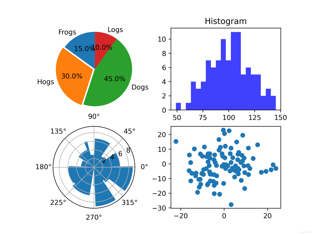
6. pyplot圖的繪製
1. 餅圖的繪製: plt.pie()
startangle:餅圖起始角度
2. 直方圖的繪製:plt.hist(x, bin)
x:此例題是一個數組,正態分佈的數組
bin:直方圖一條條長方形的個數,在數值x的值域中劃分bin個區間
橫軸是x的大小分佈,縱軸是每個值出現的次數
alpha:用於設置直方圖的透明度
3. 極座標圖繪製
4. 散點圖繪製
法一:前面介紹的plot方法繪製 -- 圖形表示方法設置成點即可
法二:面向對象的
import matplotlib.pyplot as plt
import numpy as np

# 餅圖
plt.subplot(2, 2, 1)
labels = 'Frogs', 'Hogs', 'Dogs', 'Logs'
sizes = [15, 30, 45, 10]
explode = (0, 0.05, 0, 0)
plt.pie(sizes, explode=explode, labels=labels, autopct='%1.1f%%', shadow=False, startangle=90)
plt.axis('equal')  # 是餅圖是個正方形的大小區域
# 直方圖
plt.subplot(2, 2, 2)
np.random.seed(0)
mu, sigma = 100, 20  # 均值和標準差
a = np.random.normal(mu, sigma, size=100)
plt.hist(a, 20, histtype='stepfilled', facecolor='b', alpha=0.75)
plt.title('Histogram')
# 極座標圖
ax = plt.subplot(2, 2, 3, projection='polar')
N = 20
theta = np.linspace(0.0, 2 * np.pi, N, endpoint=False)
# print(theta)  # 隨機生成了一個帶有10個數字的數組 -- left
radii = 10 * np.random.rand(N)
# print(radii)  # 隨機生成了一個帶有10個數字的數組 -- 高
width = np.pi / 4 * np.random.rand(N)
# print(width)  # 隨機生成了一個帶有10個數字的數組 -- 每個條形的角度值

bars = ax.bar(theta, height=radii, width=width)
# 散點圖
plt.subplot(2, 2, 4)
plt.plot(10*np.random.randn(100), 10*np.random.randn(100), 'o')
plt.savefig("../img_plt/P6", dpi=500)
plt.show()
運行結果:
Pandas內容
Pandas提供DataFrame數據結構,專為表格數據設計,支持數據清洗、聚合、時間序列分析等。廣泛應用於金融、統計等領域。
Pandas庫主要提供兩個數據類型:Series, DataFrame
Numpy: 基礎數據類型 | 關注數據的結構表達 | 維度:數據間關係
Pandas:擴展數據類型 | 關注數據的應用表達 | 數據與索引間的關係
1. Series類型
由一組數據和與之相關的數據索引組成
Series類型的創建:
1. Python列表創建
2. 從標量創建
3. 從字典創建
4. ndarray類型創建
Series基本操作:
1. index
2. values
3. 索引切片形式查找數據
4. in判斷是否包含某個值
5. f.get(index, data):f中有索引index,則返回索引是index的值;若不存在索引index,則返回data
6. Series對其操作:基於索引運算
7. Series對象和索引都可以由一個名字,存儲在屬性.name中 -- a.name = ''和a.index.name = ''
8. 對象可以隨時修改並即刻生效
# 列表創建
a = pd.Series([9, 8, 7, 6])
print(a)

# 自定義索引
b = pd.Series([9, 8, 7, 6], index=['a', 'b', 'c', 'd'])
print(b)

# 標量創建
c = pd.Series(25, index=['a', 'b', 'c', 'd'])
print(c)
# 從字典創建,可通過index對形狀進行規定
d = pd.Series({'a': 9, 'b': 8, 'c': 7})
print(d)
d = pd.Series({'a': 9, 'b': 8, 'c': 7}, index=['a', 'b', 'c', 'd'])
print(d)
# ndarray類型創建
e = pd.Series(np.arange(5))
print(e)
e = pd.Series(np.arange(5), index=np.arange(9, 4, -1))
print(e)

print('-----------------------')
f = pd.Series([9, 8, 7, 6], index=['a', 'b', 'c', 'd'])
print(f)
print(f.index)
print(f.values)
print(f['b'])
# print(f[1])
print(f[['a', 'b']])
# 切片索引
print(f[: 3])
# in
print('c' in f)  # True
print(0 in f)  # False
# get()
print(f.get('b', 100), f.get('e', 200))  # 8 20

# 對其操作
g = pd.Series([1, 2, 3], index=['a', 'b', 'c'])
h = pd.Series([4, 5, 6, 7], index=['b', 'c', 'd', 'e'])
print(g+h)

# .name()
i = pd.Series(np.arange(3))
i.name = 'Series對象'
i.index.name = '索引列'
print(i)
print('--------')
# 修改對象
i[0] = 10
i.name = '修改對象'
print(i)
運行結果:
0    9
1    8
2    7
3    6
dtype: int64
a    9
b    8
c    7
d    6
dtype: int64
a    25
b    25
c    25
d    25
dtype: int64
a    9
b    8
c    7
dtype: int64
a    9.0
b    8.0
c    7.0
d    NaN
dtype: float64
0    0
1    1
2    2
3    3
4    4
dtype: int64
9    0
8    1
7    2
6    3
5    4
dtype: int64
-----------------------
a    9
b    8
c    7
d    6
dtype: int64
Index(['a', 'b', 'c', 'd'], dtype='object')
[9 8 7 6]
8
a    9
b    8
dtype: int64
a    9
b    8
c    7
dtype: int64
True
False
8 200
a    NaN
b    6.0
c    8.0
d    NaN
e    NaN
dtype: float64
索引列
0    0
1    1
2    2
Name: Series對象, dtype: int64
--------
索引列
0    10
1     1
2     2
Name: 修改對象, dtype: int64

進程已結束,退出代碼0
2. DataFrame類型
DataFrame:由共同相同索引的一組列組成 -- 類似於表格
有行索引和列索引:
行索引:index -- axis=0
列索引:column -- axis=1
DataFrame類型的創建:
1. 二維ndarray對象創建
2. 一維ndarray對象字典創建
3. 列表類型的字典創建
DataFrame類型的數據獲取:
1. 列獲取:a['列名']
2. 行獲取:a.ix['行名'] -- 不可用
import pandas as pd
import numpy as np
"""
    DataFrame:由共同相同索引的一組列組成 -- 類似於表格
        有行索引和列索引:
                    行索引:index -- axis=0
                    列索引:column -- axis=1
        DataFrame類型的創建:
                    1. 二維ndarray對象創建
                    2. 一維ndarray對象字典創建
                    3. 列表類型的字典創建
        DataFrame類型的數據獲取:
                    1. 列獲取:a['列名']
                    2. 行獲取:a.ix['行名'] -- 不可用

"""
# 二維ndarray對象創建
a = pd.DataFrame(np.arange(10).reshape(2, 5))
print(a)

# 一維ndarray對象字典創建
b = {'one': pd.Series([1, 2, 3], index=['a', 'b', 'c']),
     'two': pd.Series([9, 8, 7, 6], index=['a', 'b', 'c', 'd'])}
print(b)
c = pd.DataFrame(b)
print(c)

# 列表類型的字典創建
d = {'one': [1, 2, 3], 'two': [4, 5, 6]}
e = pd.DataFrame(d, index=['a', 'b', 'c'])
print(e)

# 列獲取
print(e['one'])
# 行獲取
# print(e.loc['b'])
運行結果:
0  1  2  3  4
0  0  1  2  3  4
1  5  6  7  8  9
{'one': a    1
b    2
c    3
dtype: int64, 'two': a    9
b    8
c    7
d    6
dtype: int64}
   one  two
a  1.0    9
b  2.0    8
c  3.0    7
d  NaN    6
   one  two
a    1    4
b    2    5
c    3    6
a    1
b    2
c    3
Name: one, dtype: int64
3. 數據類型操作
如何改變Series和DataFrame對象?
增加或重排:重新索引
.reindex()能夠改變或重排Series和DataFrame索引
參數:
index,columns
fill_value:重新索引中,用於填充缺失的位置
method:填充方法,fill當前值向前填充,bfill向後填充
limit:最大值填充量
copy:默認True,生成新的對象;False時,新舊相等不復制 -- 運用不多
index索引,不可修改
索引類型的方法:
.append(idx):連接另一個Index對象,產生新的Index對象
.diff(idx):計算差集,產生新的Index對象
.intersection(idx):計算交集
.union(idx):計算並集
.delete(loc):刪除loc位置處的元素 注:delete和insert不可同時使用,分開寫,否則報錯
.insert(loc, e):在loc位置增加一個元素
刪除:drop() 刪除指定行或列索引 -- 與delete()功能一樣
刪除行:.drop('行名')
刪除列:.drop('列名', axis=1)
import pandas as pd


a = {'城市': ['北京', '上海', '廣州'],
     '環比': [1, 1, 1],
     '同比': [6, 6, 6]}
b = pd.DataFrame(a, index=['c1', 'c2', 'c3'])
print(b)

# 行的標籤順序(columns) + 列標籤順序(index)
b = b.reindex(columns=['城市', '同比', '環比'], index=['c3', 'c2', 'c1'])
print(b)

# 新增列填充
newc = b.columns.insert(3, '新增')
print(newc)
newd = b.reindex(columns=newc, fill_value=200)
print(newd)

print('---------------')
a = {'城市': ['北京', '上海', '廣州'],
     '環比': [1, 2, 3],
     '同比': [1, 2, 3]}
b = pd.DataFrame(a, index=['c1', 'c2', 'c3'])
print(b)
nc = b.columns.delete(0)
ni = b.index.insert(3, 'c4')
b = b.reindex(index=ni, method='ffill')
print(b)
c = b.reindex(columns=nc)
print(c)
# drop
c = c.drop(['c2', 'c3'])
c = c.drop('同比', axis=1)
print(c)
運行結果:
城市  環比  同比
c1  北京   1   6
c2  上海   1   6
c3  廣州   1   6
    城市  同比  環比
c3  廣州   6   1
c2  上海   6   1
c1  北京   6   1
Index(['城市', '同比', '環比', '新增'], dtype='object')
    城市  同比  環比   新增
c3  廣州   6   1  200
c2  上海   6   1  200
c1  北京   6   1  200
---------------
    城市  環比  同比
c1  北京   1   1
c2  上海   2   2
c3  廣州   3   3
    城市  環比  同比
c1  北京   1   1
c2  上海   2   2
c3  廣州   3   3
c4  廣州   3   3
    環比  同比
c1   1   1
c2   2   2
c3   3   3
c4   3   3
    環比
c1   1
c4   3
4. 數據類型運算
算數運算法則:
根據行列索引,補齊後運算,運算默認產生浮點數
補齊時缺項填充NaN(空值)
二維和一維、一維和零維間為廣播運算
採用+ - * / 符號進行的二元運算產生新的對象
可用方法: -- 優點:可選參數 -- 參數fill_value = ... 來代替NaN後進行運算
.add()
.sub()
.mul()
.div()
比較運算法則:
比較運算只能比較相同索引的元素,不進行補齊
二維和一維、一維和零維間為廣播運算 -- 不同維度運算,廣播運算,默認在1軸 -- 1軸為行,0軸為列
採用> < >= <= == !=等運算進行的二元運算產生布爾對象
import pandas as pd
import numpy as np
"""
數據類型運算
    算數運算法則:
        根據行列索引,補齊後運算,運算默認產生浮點數
        補齊時缺項填充NaN(空值)
        二維和一維、一維和零維間為廣播運算
        採用+ - * / 符號進行的二元運算產生新的對象
            可用方法: -- 優點:可選參數 -- 參數fill_value = ... 來代替NaN後進行運算
                .add()
                .sub()
                .mul()
                .div()
"""

a = pd.DataFrame(np.arange(12).reshape(3, 4))
print(a)
b = pd.DataFrame(np.arange(20).reshape(4, 5))
print(b)
# 算數+
print(a+b)
# 算數+ ,使用方法add -- a,b之間缺少的元素用100補齊,補齊之後再運算
print(a.add(b, fill_value=100))
print(a.mul(b, fill_value=0))

print("================")
"""
    不同維數的運算
"""
c = pd.DataFrame(np.arange(20).reshape(4, 5))
print(c)
d = pd.Series(np.arange(5))
print(d)
print(d - 10)
# c的每一行 - d
print(c - d)
# c的每一列 - d  --  0軸為單位運算
e = c.sub(d, axis=0)
print(e)

"""
    比較運算法則:
        比較運算只能比較相同索引的元素,不進行補齊
        二維和一維、一維和零維間為廣播運算 -- 不同維度運算,廣播運算,默認在1軸  --  1軸為行,0軸為列
        採用> < >= <= == !=等運算進行的二元運算產生布爾對象
"""
f = pd.DataFrame(np.arange(12).reshape(3, 4))
print(f)
g = pd.DataFrame(np.arange(12, 0, -1).reshape(3, 4))
print(g)
print(f > g)
print(f == g)

# 不同維度
h = pd.Series(np.arange(4))
print(h)
print(f > h)
運行結果:
0  1   2   3
0  0  1   2   3
1  4  5   6   7
2  8  9  10  11
    0   1   2   3   4
0   0   1   2   3   4
1   5   6   7   8   9
2  10  11  12  13  14
3  15  16  17  18  19
      0     1     2     3   4
0   0.0   2.0   4.0   6.0 NaN
1   9.0  11.0  13.0  15.0 NaN
2  18.0  20.0  22.0  24.0 NaN
3   NaN   NaN   NaN   NaN NaN
       0      1      2      3      4
0    0.0    2.0    4.0    6.0  104.0
1    9.0   11.0   13.0   15.0  109.0
2   18.0   20.0   22.0   24.0  114.0
3  115.0  116.0  117.0  118.0  119.0
      0     1      2      3    4
0   0.0   1.0    4.0    9.0  0.0
1  20.0  30.0   42.0   56.0  0.0
2  80.0  99.0  120.0  143.0  0.0
3   0.0   0.0    0.0    0.0  0.0
================
    0   1   2   3   4
0   0   1   2   3   4
1   5   6   7   8   9
2  10  11  12  13  14
3  15  16  17  18  19
0    0
1    1
2    2
3    3
4    4
dtype: int64
0   -10
1    -9
2    -8
3    -7
4    -6
dtype: int64
    0   1   2   3   4
0   0   0   0   0   0
1   5   5   5   5   5
2  10  10  10  10  10
3  15  15  15  15  15
      0     1     2     3     4
0   0.0   1.0   2.0   3.0   4.0
1   4.0   5.0   6.0   7.0   8.0
2   8.0   9.0  10.0  11.0  12.0
3  12.0  13.0  14.0  15.0  16.0
4   NaN   NaN   NaN   NaN   NaN
   0  1   2   3
0  0  1   2   3
1  4  5   6   7
2  8  9  10  11
    0   1   2  3
0  12  11  10  9
1   8   7   6  5
2   4   3   2  1
       0      1      2      3
0  False  False  False  False
1  False  False  False   True
2   True   True   True   True
       0      1      2      3
0  False  False  False  False
1  False  False   True  False
2  False  False  False  False
0    0
1    1
2    2
3    3
dtype: int64
       0      1      2      3
0  False  False  False  False
1   True   True   True   True
2   True   True   True   True
5. 排序
pandas排序:
.sort_index()方法在指定軸上根據索引進行排序,默認升序
參數:
axis:默認為0
ascending:默認為True -- 遞增排序
Series.sort_values()方法在指定軸上根據數值進行排序,默認升序
參數:
axis:默認為0
ascending:默認為True -- 遞增排序
DataFrame.sort_values()方法在指定軸上根據數值進行排序,默認升序
參數:
by:axis軸上的某個索引或索引列表 -- 指定以axis上的哪個列(行)為標準進行排序
axis:默認為0
ascending:默認為True -- 遞增排序
NaN空值統一放到排序的末尾
import pandas as pd
import numpy as np


a = pd.DataFrame(np.arange(20).reshape(4, 5), index=['c', 'd', 'a', 'b'])
print(a)
print(a.sort_index(axis=0, ascending=True))
print(a.sort_index(axis=0, ascending=False))

# .sort_values()
print(a.sort_values('d', axis=1, ascending=False))

# 空值排序
a = pd.DataFrame(np.arange(12).reshape(3, 4))
print(a)
b = pd.DataFrame(np.arange(20).reshape(4, 5))
print(b)
# 算數+
c = a + b
print(c)
print(c.sort_values(1, ascending=False))
運行結果:
0   1   2   3   4
c   0   1   2   3   4
d   5   6   7   8   9
a  10  11  12  13  14
b  15  16  17  18  19
    0   1   2   3   4
a  10  11  12  13  14
b  15  16  17  18  19
c   0   1   2   3   4
d   5   6   7   8   9
    0   1   2   3   4
d   5   6   7   8   9
c   0   1   2   3   4
b  15  16  17  18  19
a  10  11  12  13  14
    4   3   2   1   0
c   4   3   2   1   0
d   9   8   7   6   5
a  14  13  12  11  10
b  19  18  17  16  15
   0  1   2   3
0  0  1   2   3
1  4  5   6   7
2  8  9  10  11
    0   1   2   3   4
0   0   1   2   3   4
1   5   6   7   8   9
2  10  11  12  13  14
3  15  16  17  18  19
      0     1     2     3   4
0   0.0   2.0   4.0   6.0 NaN
1   9.0  11.0  13.0  15.0 NaN
2  18.0  20.0  22.0  24.0 NaN
3   NaN   NaN   NaN   NaN NaN
      0     1     2     3   4
2  18.0  20.0  22.0  24.0 NaN
1   9.0  11.0  13.0  15.0 NaN
0   0.0   2.0   4.0   6.0 NaN
3   NaN   NaN   NaN   NaN NaN
6. 分析
6.1. 基本統計分析
基本的統計分析函數:
.sum(): 計算數據的總和,按0軸計算,下同
.count():非NaN值的數量
.mean() .median(): 計算數據的算術平均值、算術中位數
.var() .std(): 計算數據的方差、標準差
.min() .max(): 計算數據的最小值、最大值
只適用Series類型:
.argmin() .argmax(): 計算數據最大值、最小值所在位置的索引位置(自動索引)
.idxmin() .idxmax(): 計算數據最大值、最小值所在位置的索引位置(引用索引)
適用Series和DataFrame類型:
.describe(): 針對0軸(各列)的統計彙總
a.describe()['max'] -- 獲取a中max
6.2. 累計統計分析
適用於Series和DataFrame類型: 默認axis=0
.cumsum(): 一次給出前1、2、...、n個數的和
.cumprod(): 一次給出前1、2、...、n個數的積
.cummax(): 一次給出前1、2、...、n個數的最大值
.cummin(): 一次給出前1、2、...、n個數的最小值
適用於Series和DataFrame類型,滾動計算(窗口計算):
.rolling(w).sum(): 依次計算相鄰w個元素的和
.rolling(w).mean(): 依次計算相鄰w個元素的算數平均值
.rolling(w).var(): 依次計算相鄰w個元素的方差
.rolling(w).std(): 依次計算相鄰w個元素的標準差
.rolling(w).min() max(): 依次計算相鄰w個元素的最小值和最大值
6.3. 相關分析
兩個事物,表示為X和Y,如何判斷他們之間的存在相關性?
相關性:
X增大,Y增大,兩個變量正相關
X增大,Y減小,兩個變量負相關
X增大,Y無視,兩個變量不相關
如何度量相關性:
協方差方法:
協方差>0,X和Y正相關
協方差<0,X和Y負相關
協方差=0,X和Y獨立無關
由於協方差不很精準,則提出:
Pearson相關係數r:
r的範圍:[0,1]
0.8-1.0 極強相關
0.6-0.8 強相關
0.4-0.6 中等程度相關
0.2-0.4 弱相關
0.0-0.2 極弱相關或無相關
適用於Series和DataFrame類型,分析函數:
.cov(): 計算協方差
.corr(): 計算相關係數矩陣,Pearson、Spearman、Kendall係數
實例:房價增幅與M2增幅的相關性
6.4. 實例
import pandas as pd
import numpy as np
import matplotlib.pyplot as plt


a = pd.Series([9, 8, 7, 6], index=['a', 'b', 'c', 'd'])
print(a.describe())
print(type(a.describe()))
print(a.describe()['max'])

print("=======================")
b = pd.DataFrame(np.arange(20).reshape(4, 5), index=['c', 'd', 'a', 'b'])
print(b.describe())
# print(b.describe().ix['count'])
print(b.describe()[2])
print(b.describe()[2]['max'])


print("############################")
# 統計函數
c = pd.DataFrame(np.arange(20).reshape(4, 5), index=['c', 'd', 'a', 'b'])
print(c)
print(c.cumsum())
print(c.rolling(2).sum())

print("==========================")
hprice = pd.Series([3.04, 22.93, 12.75, 22.6, 12.33], index=['2008', '2009', '2010', '2011', '2012'])
print(hprice)
m2 = pd.Series([8.18, 18.38, 9.13, 7.82, 6.69], index=['2008', '2009', '2010', '2011', '2012'])
print(m2)
print("相關性:{}".format(hprice.corr(m2)))

plt.subplot(1, 1, 1)
x = ['2008', '2009', '2010', '2011', '2012']
y1 = [3.04, 22.93, 12.75, 22.6, 12.33]
y2 = [8.18, 18.38, 9.13, 7.82, 6.69]
plt.plot(x, y1, marker='o')
plt.plot(x, y2, marker='o')
plt.show()
運行結果:
count    4.000000
mean     7.500000
std      1.290994
min      6.000000
25%      6.750000
50%      7.500000
75%      8.250000
max      9.000000
dtype: float64
<class 'pandas.core.series.Series'>
9.0
=======================
               0          1          2          3          4
count   4.000000   4.000000   4.000000   4.000000   4.000000
mean    7.500000   8.500000   9.500000  10.500000  11.500000
std     6.454972   6.454972   6.454972   6.454972   6.454972
min     0.000000   1.000000   2.000000   3.000000   4.000000
25%     3.750000   4.750000   5.750000   6.750000   7.750000
50%     7.500000   8.500000   9.500000  10.500000  11.500000
75%    11.250000  12.250000  13.250000  14.250000  15.250000
max    15.000000  16.000000  17.000000  18.000000  19.000000
count     4.000000
mean      9.500000
std       6.454972
min       2.000000
25%       5.750000
50%       9.500000
75%      13.250000
max      17.000000
Name: 2, dtype: float64
17.0
############################
    0   1   2   3   4
c   0   1   2   3   4
d   5   6   7   8   9
a  10  11  12  13  14
b  15  16  17  18  19
    0   1   2   3   4
c   0   1   2   3   4
d   5   7   9  11  13
a  15  18  21  24  27
b  30  34  38  42  46
      0     1     2     3     4
c   NaN   NaN   NaN   NaN   NaN
d   5.0   7.0   9.0  11.0  13.0
a  15.0  17.0  19.0  21.0  23.0
b  25.0  27.0  29.0  31.0  33.0
==========================
2008     3.04
2009    22.93
2010    12.75
2011    22.60
2012    12.33
dtype: float64
2008     8.18
2009    18.38
2010     9.13
2011     7.82
2012     6.69
dtype: float64
相關性:0.5239439145220387