
最新案例動態,請查閲【案例共創】基於spaCy的NER模型構建與深度EDA解析:Twitter情感短語提取。小夥伴們快來領取華為開發者空間進行實操吧!
本案例由開發者:天津師範大學協同育人項目–翟羽佳提供
1 概述
1.1 案例介紹
社交媒體已成為全球用户表達情感與觀點的重要平台,Twitter 作為典型代表,每日產生海量文本數據。情感分析作為自然語言處理的重要分支,在輿情監測、品牌口碑分析等領域發揮關鍵作用。傳統的情感分析多依賴基於規則或簡單詞袋模型,難以捕捉複雜語義與領域特定情感表達。在 Twitter 文本中,包含大量口語化、非正式的短語,精準提取這些情感短語並構建高效情感分析模型,成為提升社交媒體情感分析準確性與實用性的關鍵挑戰。 數據科學價值
本案例藉助開發者空間提供的AI Notebook進行深度文本挖掘,通過詞性標註、依存句法分析等 NLP 技術,結合 spaCy 的命名實體識別(NER)模型,精準提取情感相關短語,挖掘文本深層語義特徵。
通過實際操作,可基於spaCy構建定製化NER模型,經數據增強與模型調優,顯著提升情感分析精度;實現從海量Twitter文本中快速提取關鍵情感信息,為輿情監控、市場趨勢分析等提供高效支持,助力企業決策與公共事件分析。
1.2 適用對象
- 企業
- 個人開發者
- 高校學生
1.3 案例時間
本案例總時長預計60分鐘。
1.4 案例流程

説明:
- 配置AI Notebook和運行環境環境;
- 從OBS下載文件;
- 編輯並運行代碼;
2 華為開發者空間AI Notebook和運行環境配置
2.1 華為開發者空間AI Notebook配置
本案例中,使用華為開發者空間AI Notebook進行代碼編寫、功能實現,華為開發者空間Notebook是一款面向開發者的一站式雲端開發工具,主要用於AI開發、數據分析、模型訓練等場景。
開發者直接進入到華為開發者空間工作台。
進入到華為開發者空間工作台後,找打AI Notebook,點擊立即前往。

進入到AI Notebook頁面後,選擇NPU環境點擊立即啓動。

稍等片刻後點擊查看Notebook,前往Notebook主頁面。

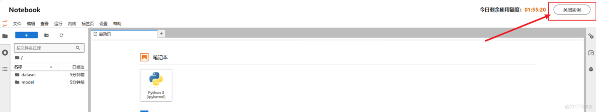
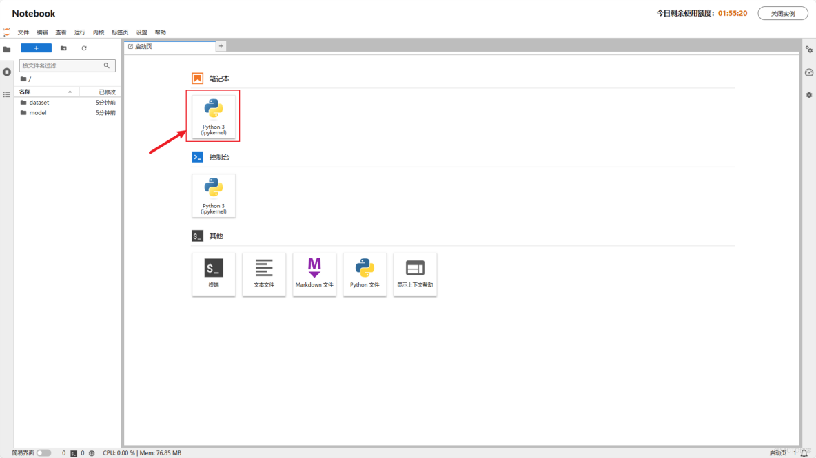
至此,成功打開Notebook。
2.2 運行環境配置
打開Notebook後,點擊筆記下的python 3,創建代碼編寫文件。
安裝第三方庫:
pip install numpy

pip install pandas

pip install matplotlib

pip install seaborn

pip install plotly

pip install pillow

pip install wordcloud

pip install nltk

pip install tqdm

pip install spacy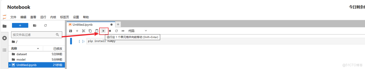
注意,如果安裝失敗可以使用國內鏡像和最新庫名進行安裝:
pip install -i https://pypi.tuna.tsinghua.edu.cn/simple numpy pandas matplotlib seaborn plotly pillow wordcloud nltk tqdm spacy系統會自動安裝相關的包和工具,當安裝完成後,系統會返回所有已成功安裝的庫,如下圖所示:
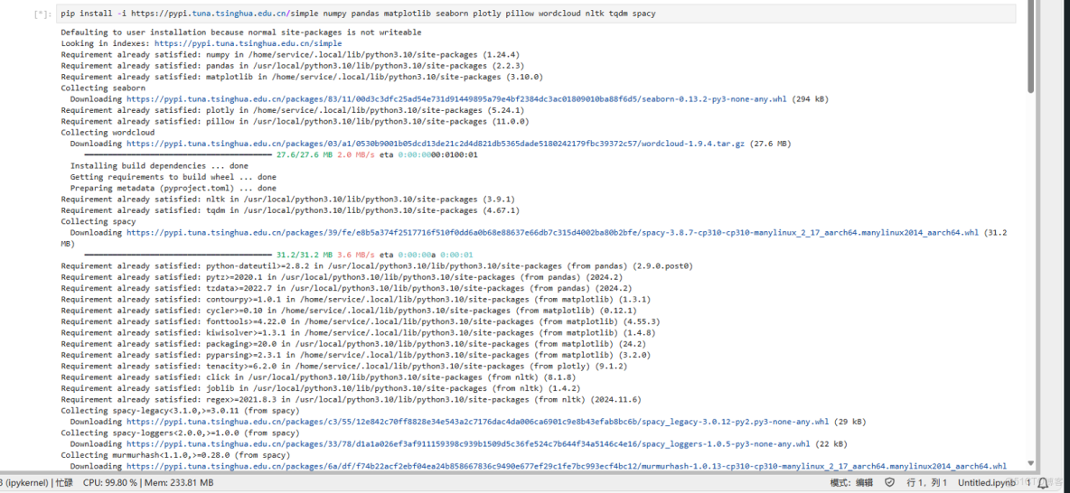
安裝成功後對腳本進行運行可得到關於 Python 數據處理全流程開發,並具備將本地模型遷移至華為雲實現工業級部署的能力。
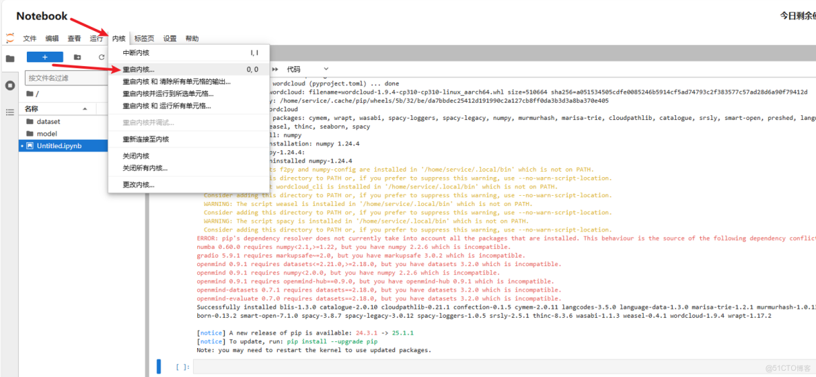
注意,安裝包安裝完畢後需要手動重啓內核來更新環境,點擊內核\>重啓內核。
3 從OBS下載文件
3.1 從obs下載所需要的文件
為了方便項目運行,已提前將文件上傳OBS,之後通過分享鏈接在Notebook中可直接下載使用。
文件壓縮包中包含後續所有的文件:
OBS鏈接地址:<https://case-aac4.obs.cn-north-4.myhuaweicloud.com/data%26models.zip >
下載命令行:
!wget <https://case-aac4.obs.cn-north-4.myhuaweicloud.com/data%26models.zip%20>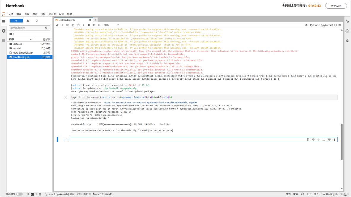
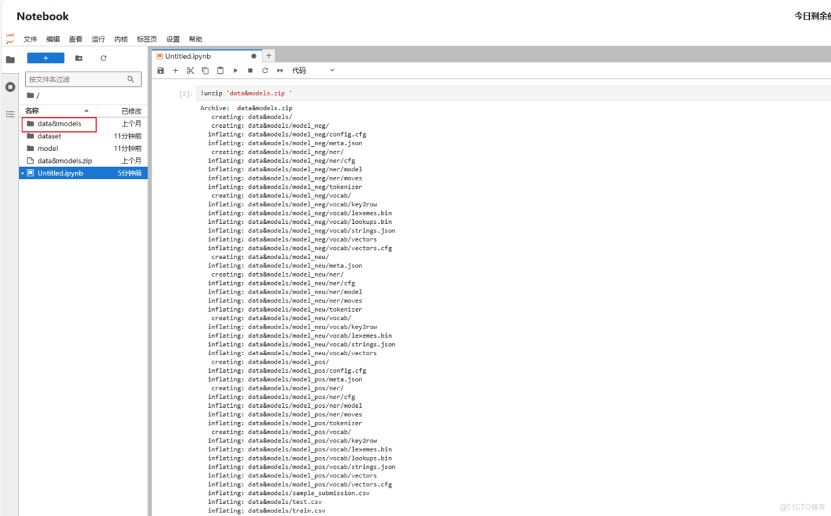
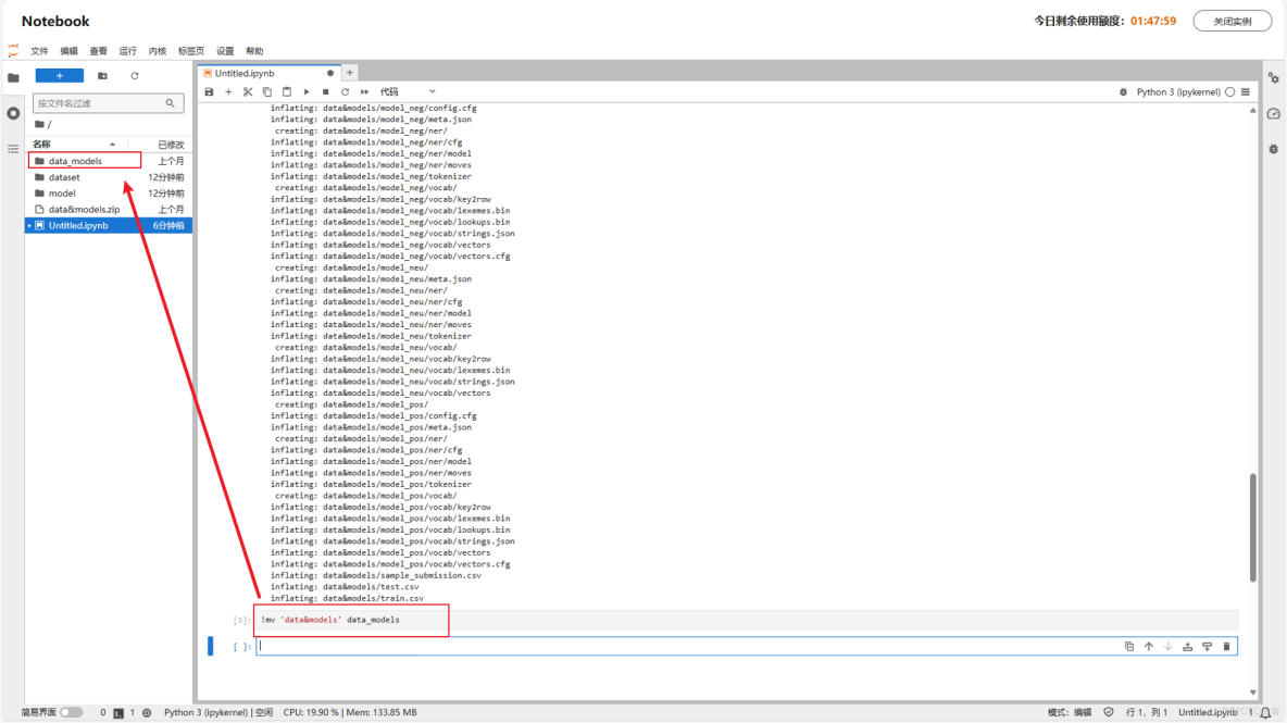
解壓壓縮包並重命名:
!unzip 'data&models.zip'!mv 'data&models' data_models注:若需使用字面意義的&,需用引號或反斜槓轉義,這裏為避免歧義,進行了重命名
4 編輯並運行代碼
4.1 複製代碼進入Notebook
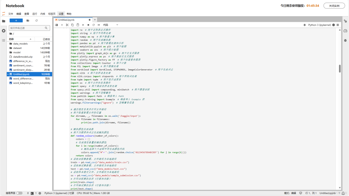
總代碼展示,直接複製到Notebook:
# 導入所需的庫
import re # 用於正則表達式操作
import string # 用於字符串處理
import numpy as np # 用於數值計算
import random # 用於生成隨機數
import pandas as pd # 用於數據處理和分析
import matplotlib.pyplot as plt # 用於繪圖
import seaborn as sns # 用於統計繪圖
from plotly import graph_objs as go # 用於交互式圖表
import plotly.express as px # 用於高級交互式圖表
import plotly.figure_factory as ff # 用於創建複雜圖表
from collections import Counter # 用於計數
from PIL import Image # 用於圖像處理
from wordcloud import WordCloud, STOPWORDS, ImageColorGenerator # 用於生成詞雲
import nltk # 用於自然語言處理
from nltk.corpus import stopwords # 用於停用詞處理
from tqdm import tqdm # 用於顯示進度條
import os # 用於文件和目錄操作
import spacy # 用於高級自然語言處理
from spacy.util import compounding, minibatch # 用於模型訓練
import warnings # 用於忽略警告
from pathlib import Path # 確保導入 Path
from spacy.training import Example # 確保導入 Example 類
warnings.filterwarnings("ignore") # 忽略警告信息
# 遍歷指定目錄並打印文件路徑
# 用於檢查數據文件的位置
for dirname, _, filenames in os.walk('/kaggle/input'):
for filename in filenames:
print(os.path.join(dirname, filename))
# 隨機顏色生成函數
# 用於為圖表和詞雲生成隨機顏色
def random_colours(number_of_colors):
colors = []
# 生成指定數量的隨機顏色
for i in range(number_of_colors):
# 隨機選擇十六進制字符生成顏色代碼
colors.append("#"+''.join([random.choice('0123456789ABCDEF') for j in range(6)]))
return colors
# 讀取訓練集數據,文件路徑為本地路徑
train = pd.read_csv(r"data_models/train.csv")
# 讀取測試集數據,文件路徑為本地路徑
test = pd.read_csv(r"data_models/test.csv")
# 讀取樣本提交文件,文件路徑為本地路徑
ss = pd.read_csv(r"data_models/sample_submission.csv")
# 打印訓練集的形狀(行數和列數)
print(train.shape)
# 打印測試集的形狀(行數和列數)
print(test.shape)
train.dropna(inplace=True)
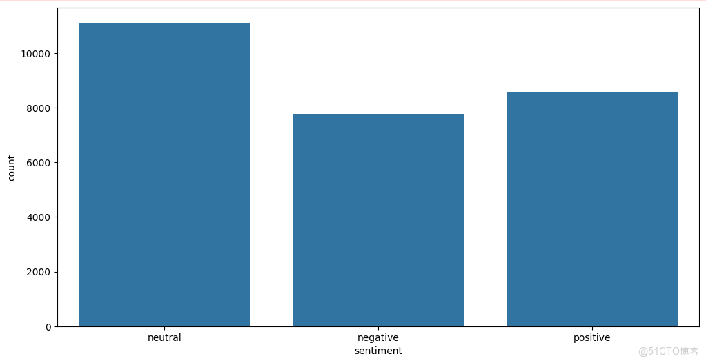
# 按情感類別(sentiment)對訓練集進行分組,統計每種情感類別的推文數量,並按數量降序排列
temp = train.groupby('sentiment').count()['text'].reset_index().sort_values(by='text', ascending=False)
# 為 temp DataFrame 添加背景漸變效果,使用紫色調(Purples)
temp.style.background_gradient(cmap='Purples')
# 創建一個大小為 12x6 英寸的 Matplotlib 圖表
plt.figure(figsize=(12, 6))
# 使用 Seaborn 繪製情感類別的柱狀圖,x 軸為不同的情感類別
sns.countplot(x='sentiment', data=train)
# 保存圖片到本地,你可以修改保存路徑和文件名
save_path = 'sentiment_countplot.png'
plt.savefig(save_path, dpi=300, bbox_inches='tight')
# 定義 Jaccard 相似度計算函數
# Jaccard 相似度用於衡量兩個集合的相似程度,取值範圍在 0 到 1 之間,值越接近 1 表示兩個集合越相似
def jaccard(str1, str2):
# 將字符串轉換為小寫,並按空格分割成單詞列表,再轉換為集合
a = set(str1.lower().split())
b = set(str2.lower().split())
# 計算兩個集合的交集
c = a.intersection(b)
# 計算 Jaccard 相似度得分,公式為交集元素個數除以並集元素個數
return float(len(c)) / (len(a) + len(b) - len(c))
# 初始化一個空列表,用於存儲計算得到的 Jaccard 相似度結果
results_jaccard = []
# 遍歷訓練集的每一行
for ind, row in train.iterrows():
# 獲取當前行的 text 列的值作為第一個句子
sentence1 = row.text
# 獲取當前行的 selected_text 列的值作為第二個句子
sentence2 = row.selected_text
# 調用 jaccard 函數計算兩個句子的 Jaccard 相似度得分
jaccard_score = jaccard(sentence1, sentence2)
# 將兩個句子和對應的 Jaccard 相似度得分添加到結果列表中
results_jaccard.append([sentence1, sentence2, jaccard_score])
# 將存儲 Jaccard 相似度結果的列表轉換為 DataFrame
jaccard = pd.DataFrame(results_jaccard, columns=["text", "selected_text", "jaccard_score"])
# 將包含 Jaccard 相似度得分的 DataFrame 與訓練集進行外連接合並
train = train.merge(jaccard, how='outer')
# 計算訓練集中 selected_text 列每個文本的單詞數量,並將結果存儲在新列 Num_words_ST 中
train['Num_words_ST'] = train['selected_text'].apply(lambda x: len(str(x).split()))
# 計算訓練集中 text 列每個文本的單詞數量,並將結果存儲在新列 Num_word_text 中
train['Num_word_text'] = train['text'].apply(lambda x: len(str(x).split()))
# 計算訓練集中 text 列和 selected_text 列單詞數量的差值,並將結果存儲在新列 difference_in_words 中
train['difference_in_words'] = train['Num_word_text'] - train['Num_words_ST']
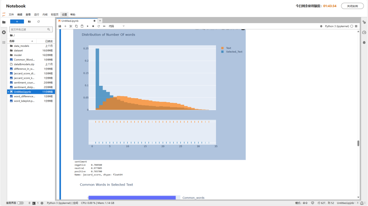
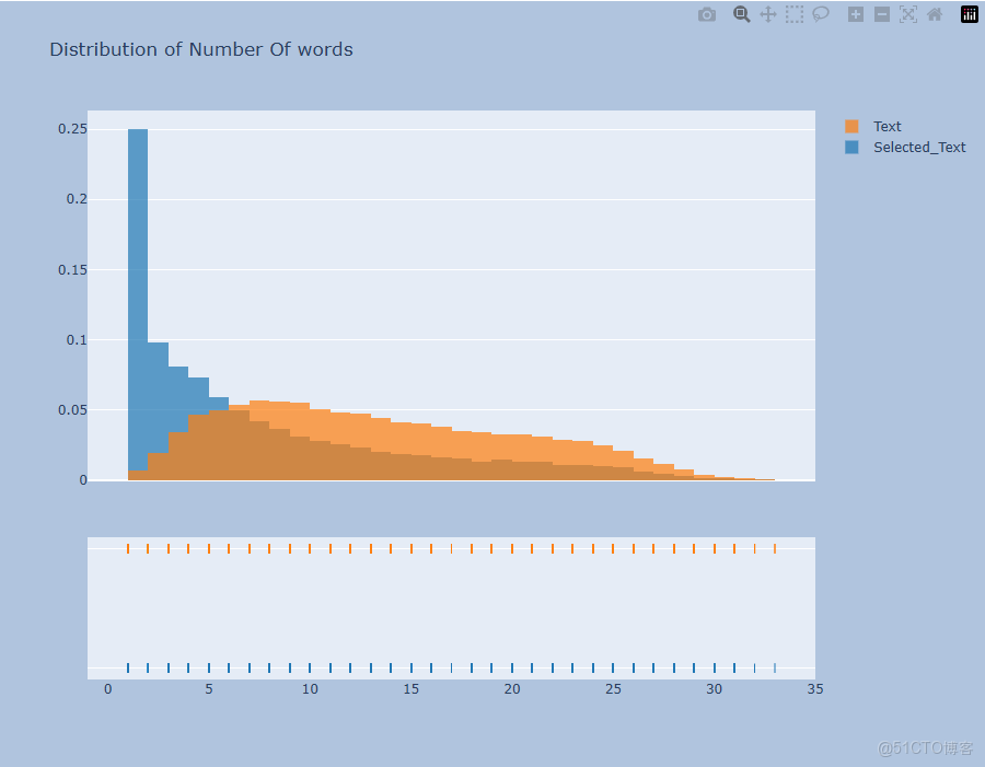
# 提取訓練集中 Num_words_ST 列和 Num_word_text 列的數據,用於繪製分佈直方圖
hist_data = [train['Num_words_ST'], train['Num_word_text']]
# 為直方圖中的不同數據集設置標籤
group_labels = ['Selected_Text', 'Text']
# 使用 Plotly 的 create_distplot 函數創建分佈直方圖,不顯示曲線
fig = ff.create_distplot(hist_data, group_labels, show_curve=False)
# 設置直方圖的標題
fig.update_layout(title_text='Distribution of Number Of words')
# 設置圖形的大小和背景顏色
fig.update_layout(
autosize=False,
width=900,
height=700,
paper_bgcolor="LightSteelBlue",
)
# 顯示繪製好的直方圖
fig.show()
# 保存圖片到本地,你可以修改保存路徑和文件名
save_path = 'sentiment_distplot.png'
plt.savefig(save_path, dpi=300, bbox_inches='tight')
# 設置圖形的大小
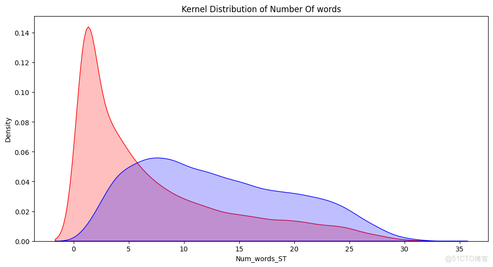
plt.figure(figsize=(12, 6))
# 使用 Seaborn 繪製訓練集 Num_words_ST 列的核密度估計圖,設置陰影和顏色為紅色,並設置標題
p1 = sns.kdeplot(train['Num_words_ST'], shade=True, color="r").set_title('Kernel Distribution of Number Of words')
# 使用 Seaborn 繪製訓練集 Num_word_text 列的核密度估計圖,設置陰影和顏色為藍色
p1 = sns.kdeplot(train['Num_word_text'], shade=True, color="b")
# 保存圖片到本地,你可以修改保存路徑和文件名
save_path = 'word_kdeplot.png'
plt.savefig(save_path, dpi=300, bbox_inches='tight')
# 設置圖形的大小
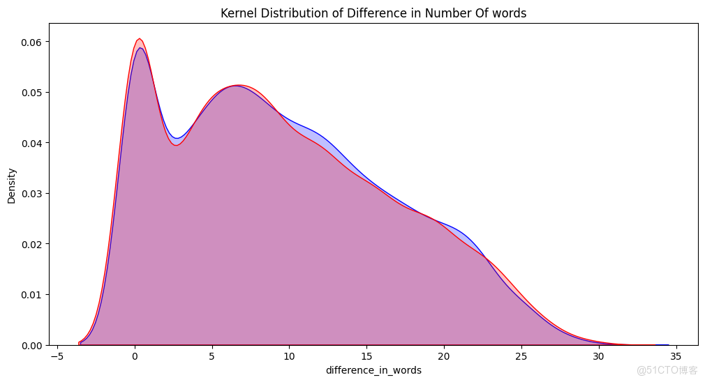
plt.figure(figsize=(12, 6))
# 篩選出訓練集中情感為 positive 的數據,繪製 difference_in_words 列的核密度估計圖,設置陰影和顏色為藍色,並設置標題
p1 = sns.kdeplot(train[train['sentiment'] == 'positive']['difference_in_words'], shade=True, color="b").set_title('Kernel Distribution of Difference in Number Of words')
# 篩選出訓練集中情感為 negative 的數據,繪製 difference_in_words 列的核密度估計圖,設置陰影和顏色為紅色
p2 = sns.kdeplot(train[train['sentiment'] == 'negative']['difference_in_words'], shade=True, color="r")
# 保存圖片到本地,你可以修改保存路徑和文件名
save_path = 'word_difference_kdeplot.png'
plt.savefig(save_path, dpi=300, bbox_inches='tight')
# 設置圖形的大小
plt.figure(figsize=(12, 6))
# 篩選出訓練集中情感為 neutral 的數據,繪製 difference_in_words 列的分佈直方圖,不顯示核密度曲線
sns.distplot(train[train['sentiment'] == 'neutral']['difference_in_words'], kde=False)
# 保存圖片到本地,你可以修改保存路徑和文件名
save_path = 'difference_in_words_distplot.png'
plt.savefig(save_path, dpi=300, bbox_inches='tight')
# 設置圖形的大小
plt.figure(figsize=(12, 6))
# 篩選出訓練集中情感為 positive 的數據,繪製 jaccard_score 列的核密度估計圖,設置陰影和顏色為藍色,並設置標題
p1 = sns.kdeplot(train[train['sentiment'] == 'positive']['jaccard_score'], shade=True, color="b").set_title('KDE of Jaccard Scores across different Sentiments')
# 篩選出訓練集中情感為 negative 的數據,繪製 jaccard_score 列的核密度估計圖,設置陰影和顏色為紅色
p2 = sns.kdeplot(train[train['sentiment'] == 'negative']['jaccard_score'], shade=True, color="r")
# 添加圖例,顯示 positive 和 negative 對應的曲線
plt.legend(labels=['positive', 'negative'])
# 保存圖片到本地,你可以修改保存路徑和文件名
save_path = 'jaccard_score_kdeplot.png'
plt.savefig(save_path, dpi=300, bbox_inches='tight')
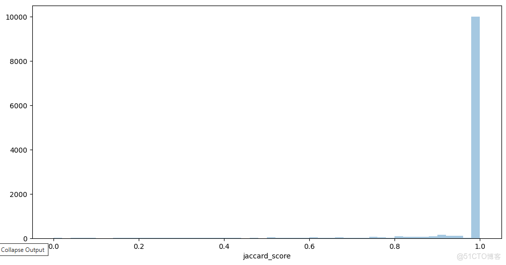
# 設置圖形的大小
plt.figure(figsize=(12, 6))
# 篩選出訓練集中情感為 neutral 的數據,繪製 jaccard_score 列的分佈直方圖,不顯示核密度曲線
sns.distplot(train[train['sentiment'] == 'neutral']['jaccard_score'], kde=False)
# 保存圖片到本地,你可以修改保存路徑和文件名
save_path = 'jaccard_score_distplot.png'
plt.savefig(save_path, dpi=300, bbox_inches='tight')
# 從 train 數據集中篩選出 'Num_word_text' 列的值小於等於 2 的行,並將結果存儲在變量 k 中
k = train[train['Num_word_text'] <= 2]
# 從數據集 k 中選擇 'sentiment' 和 'jaccard_score' 兩列,並將結果存儲在變量 jaccard_scores 中
jaccard_scores = k[['sentiment', 'jaccard_score']]
# 按 'sentiment' 列對數據集 jaccard_scores 進行分組,並計算每組的 'jaccard_score' 列的均值
# 最後從分組結果中提取 'jaccard_score' 列的均值,並將結果存儲在變量 result 中
result = jaccard_scores.groupby('sentiment').mean()['jaccard_score']
# 打印變量 result 的值,即每個情感類別的平均 Jaccard 分數
print(result)
# 從數據集 k 中篩選出 'sentiment' 列的值等於 'positive' 的行,以便進一步分析
k[k['sentiment'] == 'positive']
def clean_text(text):
# 將文本轉換為小寫
text = str(text).lower()
# 移除方括號內的文本(例如:[...])
text = re.sub('\[.*?\]', '', text)
# 移除鏈接(包含http、https或www開頭的URL)
text = re.sub('https?://\S+|www\.\S+', '', text)
# 移除HTML標籤(例如:<br />)
text = re.sub('<.*?>+', '', text)
# 移除標點符號
text = re.sub('[%s]' % re.escape(string.punctuation), '', text)
# 移除換行符
text = re.sub('\n', '', text)
# 移除包含數字的單詞
text = re.sub('\w*\d\w*', '', text)
# 返回清洗後的文本
return text
# 對 train 數據集的 'text' 列應用 clean_text 函數,清洗文本
train['text'] = train['text'].apply(lambda x: clean_text(x))
# 對 train 數據集的 'selected_text' 列應用 clean_text 函數,清洗文本
train['selected_text'] = train['selected_text'].apply(lambda x: clean_text(x))
# 為每個 'selected_text' 的值創建一個單詞列表(按空格分割)
train['temp_list'] = train['selected_text'].apply(lambda x: str(x).split())
# 使用列表推平操作,將所有子列表中的單詞放入一個單一的列表中
top = Counter([item for sublist in train['temp_list'] for item in sublist])
# 將最常見的 20 個單詞及其出現次數轉換為 DataFrame
temp = pd.DataFrame(top.most_common(20))
# 為 DataFrame 的兩列命名
temp.columns = ['Common_words', 'count']
# 為 DataFrame 添加一個漸變顏色背景,使用藍色調
temp.style.background_gradient(cmap='Blues')
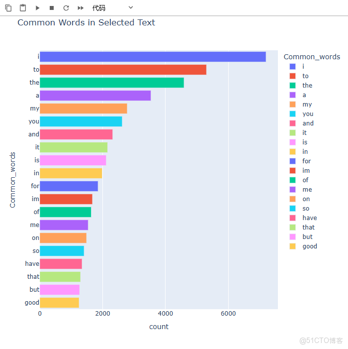
# 使用 Plotly 創建一個水平條形圖,展示最常見的單詞及其計數
fig = px.bar(temp, x="count", y="Common_words", title='Common Words in Selected Text', orientation='h',
width=700, height=700, color='Common_words')
fig.show()
# 保存圖片到本地,你可以修改保存路徑和文件名
save_path = 'Common_Words_barplot.png'
plt.savefig(save_path, dpi=300, bbox_inches='tight')
# 定義一個函數,用於移除輸入列表中的停用詞(英文)
def remove_stopword(x):
return [y for y in x if y not in stopwords.words('english')]
# 應用 remove_stopword 函數到 'temp_list' 列,移除列表中的所有英文停用詞
train['temp_list'] = train['temp_list'].apply(lambda x: remove_stopword(x))
# 再次統計移除停用詞後的所有單詞,並找出最常見的 20 個單詞
top = Counter([item for sublist in train['temp_list'] for item in sublist])
# 創建一個新的 DataFrame,包含最常見的 20 個單詞及其計數
temp = pd.DataFrame(top.most_common(20))
# 刪除 DataFrame 的第一行(通常是停用詞)
temp = temp.iloc[1:, :]
# 為 DataFrame 的兩列命名
temp.columns = ['Common_words', 'count']
# 為 DataFrame 添加一個漸變顏色背景,使用紫色調
temp.style.background_gradient(cmap='Purples')
# 使用 Plotly 創建一個樹狀圖,展示最常見的單詞及其計數
fig = px.treemap(temp, path=['Common_words'], values='count', title='Tree of Most Common Words')
fig.show()
# 保存圖片到本地,你可以修改保存路徑和文件名
save_path = 'Common_Words_treemap.png'
plt.savefig(save_path, dpi=300, bbox_inches='tight')
# 為每個 'text' 的值創建一個單詞列表(按空格分割)
train['temp_list1'] = train['text'].apply(lambda x: str(x).split())
# 應用 remove_stopword 函數到 'temp_list1' 列,移除列表中的所有英文停用詞
train['temp_list1'] = train['temp_list1'].apply(lambda x: remove_stopword(x))
# 使用列表推平操作,將所有子列表中的單詞放入一個單一的列表中
top = Counter([item for sublist in train['temp_list1'] for item in sublist])
# 將最常見的 25 個單詞及其出現次數轉換為 DataFrame
temp = pd.DataFrame(top.most_common(25))
# 刪除 DataFrame 的第一行(通常是停用詞)
temp = temp.iloc[1:, :]
# 為 DataFrame 的兩列命名
temp.columns = ['Common_words', 'count']
# 為 DataFrame 添加一個漸變顏色背景,使用藍色調
temp.style.background_gradient(cmap='Blues')
# 使用 Plotly 的 bar 函數創建一個水平條形圖
fig = px.bar(
temp, # 數據來源,即包含單詞及其計數的 DataFrame
x="count", # 橫軸為單詞的計數
y="Common_words", # 縱軸為最常見的單詞
title='Common Words in Text', # 圖表標題
orientation='h', # 設置為水平條形圖
width=700, # 圖表的寬度設置為 700 像素
height=700, # 圖表的高度設置為 700 像素
color='Common_words' # 按單詞對條形進行顏色編碼
)
# 顯示創建的圖表
fig.show()
# 保存圖片到本地,你可以修改保存路徑和文件名
save_path = 'Common_Words_barplot.png'
plt.savefig(save_path, dpi=300, bbox_inches='tight')
# 篩選出情感類別為正面(positive)的推文
Positive_sent = train[train['sentiment'] == 'positive']
# 篩選出情感類別為負面(negative)的推文
Negative_sent = train[train['sentiment'] == 'negative']
# 篩選出情感類別為中性(neutral)的推文
Neutral_sent = train[train['sentiment'] == 'neutral']
# ******************* 最常見的正面詞彙 *******************
# 使用列表推平操作,將所有子列表中的單詞放入一個單一的列表中
top = Counter([item for sublist in Positive_sent['temp_list'] for item in sublist])
# 將最常見的 20 個正面單詞及其出現次數轉換為 DataFrame
temp_positive = pd.DataFrame(top.most_common(20))
# 為 DataFrame 的兩列命名
temp_positive.columns = ['Common_words', 'count']
# 為 DataFrame 添加一個漸變顏色背景,使用綠色調
temp_positive.style.background_gradient(cmap='Greens')
# 使用 Plotly 創建一個水平條形圖,展示最常見的正面單詞及其計數
fig = px.bar(
temp_positive, # 數據來源,即常見的正面單詞及其計數
x="count", # 橫軸為單詞的計數
y="Common_words", # 縱軸為最常見的單詞
title='Most Common Positive Words', # 圖表標題
orientation='h', # 設置為水平條形圖
width=700, # 圖表的寬度設置為 700 像素
height=700, # 圖表的高度設置為 700 像素
color='Common_words' # 按單詞對條形進行顏色編碼
)
fig.show() # 顯示圖表
# 保存圖片到本地,你可以修改保存路徑和文件名
save_path = 'Positive_Words_barplot.png'
plt.savefig(save_path, dpi=300, bbox_inches='tight')
# ******************* 最常見的負面詞彙 *******************
# 使用列表推平操作,將所有子列表中的單詞放入一個單一的列表中
top = Counter([item for sublist in Negative_sent['temp_list'] for item in sublist])
# 將最常見的 20 個負面單詞及其出現次數轉換為 DataFrame
temp_negative = pd.DataFrame(top.most_common(20))
# 刪除 DataFrame 的第一行(通常是停用詞)
temp_negative = temp_negative.iloc[1:, :]
# 為 DataFrame 的兩列命名
temp_negative.columns = ['Common_words', 'count']
# 為 DataFrame 添加一個漸變顏色背景,使用紅色調
temp_negative.style.background_gradient(cmap='Reds')
# 使用 Plotly 創建一個樹狀圖,展示最常見的負面單詞及其計數
fig = px.treemap(
temp_negative, # 數據來源,即常見的負面單詞及其計數
path=['Common_words'], # 確定樹狀圖的層次結構
values='count', # 數據值,即單詞的計數
title='Tree Of Most Common Negative Words' # 圖表標題
)
fig.show() # 顯示圖表
# 保存圖片到本地,你可以修改保存路徑和文件名
save_path = 'Negative_Words_treemap.png'
plt.savefig(save_path, dpi=300, bbox_inches='tight')
# ******************* 最常見的中性詞彙 *******************
# 使用列表推平操作,將所有子列表中的單詞放入一個單一的列表中
top = Counter([item for sublist in Neutral_sent['temp_list'] for item in sublist])
# 將最常見的 20 箇中性單詞及其出現次數轉換為 DataFrame
temp_neutral = pd.DataFrame(top.most_common(20))
# 刪除 DataFrame 的第一行(通常是停用詞)
temp_neutral = temp_neutral.loc[1:, :]
# 為 DataFrame 的兩列命名
temp_neutral.columns = ['Common_words', 'count']
# 為 DataFrame 添加一個漸變顏色背景,使用紅色調
temp_neutral.style.background_gradient(cmap='Reds')
# 使用 Plotly 創建一個水平條形圖,展示最常見的中性單詞及其計數
fig = px.bar(
temp_neutral, # 數據來源,即常見的中性單詞及其計數
x="count", # 橫軸為單詞的計數
y="Common_words", # 縱軸為最常見的單詞
title='Most Common Neutral Words', # 圖表標題
orientation='h', # 設置為水平條形圖
width=700, # 圖表的寬度設置為 700 像素
height=700, # 圖表的高度設置為 700 像素
color='Common_words' # 按單詞對條形進行顏色編碼
)
fig.show() # 顯示圖表
# 保存圖片到本地,你可以修改保存路徑和文件名
save_path = 'Neutral_Words_barplot.png'
plt.savefig(save_path, dpi=300, bbox_inches='tight')
# 使用 Plotly 創建一個樹狀圖,展示最常見的中性單詞及其計數
fig = px.treemap(
temp_neutral, # 數據來源,即常見的中性單詞及其計數
path=['Common_words'], # 確定樹狀圖的層次結構
values='count', # 數據值,即單詞的計數
title='Tree Of Most Common Neutral Words' # 圖表標題
)
fig.show() # 顯示圖表
# 保存圖片到本地,你可以修改保存路徑和文件名
save_path = 'Neutral_Words_treemap.png'
plt.savefig(save_path, dpi=300, bbox_inches='tight')
# 創建一個包含所有單詞的列表,每個單詞來自 train['temp_list1'] 列中的每個子列表
raw_text = [word for word_list in train['temp_list1'] for word in word_list]
def words_unique(sentiment, numwords, raw_words):
# 收集所有不屬於當前情感類別的單詞
allother = []
for item in train[train.sentiment != sentiment]['temp_list1']:
for word in item:
allother.append(word)
allother = list(set(allother)) # 去重
# 找出在當前情感類別中特有的單詞
specificnonly = [x for x in raw_text if x not in allother]
# 統計當前情感類別中所有單詞的出現次數
mycounter = Counter()
for item in train[train.sentiment == sentiment]['temp_list1']:
for word in item:
mycounter[word] += 1
# 只保留那些在當前情感類別中特有的單詞
keep = list(specificnonly)
for word in list(mycounter):
if word not in keep:
del mycounter[word]
# 將結果轉換為數據框,並選擇出現次數最多的前 numwords 個單詞
Unique_words = pd.DataFrame(mycounter.most_common(numwords), columns=['words', 'count'])
return Unique_words
# 調用函數,獲取情感類別為 'positive' 的前 20 個獨特單詞
Unique_Positive = words_unique('positive', 20, raw_text)
print("The top 20 unique words in Positive Tweets are:")
Unique_Positive.style.background_gradient(cmap='Greens') # 添加漸變背景顏色
# 使用 Plotly 創建樹狀圖,展示積極情感類別中的獨特單詞
fig = px.treemap(Unique_Positive, path=['words'], values='count', title='Tree Of Unique Positive Words')
fig.show()
# 保存圖片到本地,你可以修改保存路徑和文件名
save_path = 'Unique_Positive_Words_treemap.png'
plt.savefig(save_path, dpi=300, bbox_inches='tight')
# 使用 Matplotlib 創建甜甜圈圖,展示積極情感類別中的獨特單詞
import palettable.colorbrewer.qualitative
plt.figure(figsize=(16, 10))
my_circle = plt.Circle((0, 0), 0.7, color='white') # 創建一個白色的圓形,用於甜甜圈圖的中心
plt.pie(Unique_Positive['count'], labels=Unique_Positive.words, colors=Pastel1_7.hex_colors) # 繪製餅圖
p = plt.gcf()
p.gca().add_artist(my_circle) # 將白色圓形添加到圖表中
plt.title('DoNut Plot Of Unique Positive Words') # 添加標題
plt.show()
# 保存圖片到本地,你可以修改保存路徑和文件名
save_path = 'Unique_Positive_Words_colorbrewer.png'
plt.savefig(save_path, dpi=300, bbox_inches='tight')
# 調用函數,獲取情感類別為 'negative' 的前 10 個獨特單詞
Unique_Negative = words_unique('negative', 10, raw_text)
print("The top 10 unique words in Negative Tweets are:")
Unique_Negative.style.background_gradient(cmap='Reds') # 添加漸變背景顏色
# 使用 Matplotlib 創建甜甜圈圖,展示消極情感類別中的獨特單詞
plt.figure(figsize=(16, 10))
my_circle = plt.Circle((0, 0), 0.7, color='white') # 創建一個白色的圓形,用於甜甜圈圖的中心
plt.rcParams['text.color'] = 'black' # 設置文本顏色為黑色
plt.pie(Unique_Negative['count'], labels=Unique_Negative.words, colors=Pastel1_7.hex_colors) # 繪製餅圖
p = plt.gcf()
p.gca().add_artist(my_circle) # 將白色圓形添加到圖表中
plt.title('DoNut Plot Of Unique Negative Words') # 添加標題
plt.show()
# 保存圖片到本地,你可以修改保存路徑和文件名
save_path = 'Unique_Negative_Words_colorbrewer.png'
plt.savefig(save_path, dpi=300, bbox_inches='tight')
# 調用函數,獲取情感類別為 'neutral' 的前 10 個獨特單詞
Unique_Neutral = words_unique('neutral', 10, raw_text)
print("The top 10 unique words in Neutral Tweets are:")
Unique_Neutral.style.background_gradient(cmap='Oranges') # 添加漸變背景顏色
# 使用 Matplotlib 創建甜甜圈圖,展示中性情感類別中的獨特單詞
plt.figure(figsize=(16, 10))
my_circle = plt.Circle((0, 0), 0.7, color='white') # 創建一個白色的圓形,用於甜甜圈圖的中心
plt.pie(Unique_Neutral['count'], labels=Unique_Neutral.words, colors=Pastel1_7.hex_colors) # 繪製餅圖
p = plt.gcf()
p.gca().add_artist(my_circle) # 將白色圓形添加到圖表中
plt.title('DoNut Plot Of Unique Neutral Words') # 添加標題
plt.show()
# 保存圖片到本地,你可以修改保存路徑和文件名
save_path = 'Unique_Neutral_Words_colorbrewer.png'
plt.savefig(save_path, dpi=300, bbox_inches='tight')
def plot_wordcloud(text, mask=None, max_words=200, max_font_size=100, figure_size=(24.0, 16.0), color='white',
title=None, title_size=40, image_color=False):
# 導入默認的停用詞
stopwords = set(STOPWORDS)
# 自定義額外的停用詞(如 'u' 和 'im')
more_stopwords = {'u', "im"}
stopwords = stopwords.union(more_stopwords)
# 創建 WordCloud 對象
wordcloud = WordCloud(
background_color=color, # 設置背景顏色
stopwords=stopwords, # 使用自定義的停用詞列表
max_words=max_words, # 控制詞雲中顯示的最大單詞數
max_font_size=max_font_size, # 控制詞雲中字體的最大大小
random_state=42, # 設置隨機種子以確保結果可復現
width=400, # 設置詞雲的寬度
height=200, # 設置詞雲的高度
)
# 使用生成所有單詞的文字(字符串)來生成詞雲
wordcloud.generate(str(text))
# 設置圖表大小
plt.figure(figsize=figure_size)
plt.title(title, fontdict={'size': title_size, 'color': 'black', 'verticalalignment': 'bottom'}) # 添加標題
plt.axis('off') # 隱藏座標軸
plt.tight_layout() # 調整佈局
# 調用 plot_wordcloud 函數,生成中性情感類別的詞雲
plot_wordcloud(Neutral_sent.text, color='white', max_font_size=100, title_size=30, title="WordCloud of Neutral Tweets")
# 保存圖片到本地,你可以修改保存路徑和文件名
save_path = 'Neutral_Words_wordcloud.png'
plt.savefig(save_path, dpi=300, bbox_inches='tight')
# 調用 plot_wordcloud 函數,生成積極情感類別的詞雲
plot_wordcloud(Positive_sent.text, title="Word Cloud Of Positive tweets", title_size=30)
# 保存圖片到本地,你可以修改保存路徑和文件名
save_path = 'Positive_Words_wordcloud.png'
plt.savefig(save_path, dpi=300, bbox_inches='tight')
# 調用 plot_wordcloud 函數,生成消極情感類別的詞雲
plot_wordcloud(Negative_sent.text, title="Word Cloud of Negative Tweets", color='white', title_size=30)
# 保存圖片到本地,你可以修改保存路徑和文件名
save_path = 'Negative_Words_wordcloud.png'
plt.savefig(save_path, dpi=300, bbox_inches='tight')
# 讀取訓練數據、測試數據和提交示例數據
df_train = pd.read_csv(r"data_models/train.csv") # 讀取訓練數據
df_test = pd.read_csv(r"data_models/test.csv") # 讀取測試數據
df_submission = pd.read_csv(r"data_models/sample_submission.csv") # 讀取提交示例數據
# 添加一列 'Num_words_text',表示每條文本的單詞數量
df_train['Num_words_text'] = df_train['text'].apply(lambda x: len(str(x).split()))
# 篩選掉單詞數量少於3的文本,以減少噪聲數據
df_train = df_train[df_train['Num_words_text'] >= 3]
# 定義保存模型的函數
def save_model(output_dir, nlp, new_model_name):
# 動態獲取桌面路徑
output_dir = os.path.expanduser(f"~/Desktop/{output_dir}")
if output_dir is not None:
# 如果路徑不存在,則創建路徑
if not os.path.exists(output_dir):
os.makedirs(output_dir)
# 設置模型的元數據名稱
nlp.meta["name"] = new_model_name
# 保存模型到指定路徑
nlp.to_disk(output_dir)
print("Saved model to", output_dir)
# 定義訓練模型的函數
def train(train_data, output_dir, n_iter=3, model=None):
# 如果提供了現有模型路徑,則加載該模型
if model is not None:
nlp = spacy.load(model) # 加載現有的 spaCy 模型
print("Loaded model '%s'" % model) # 打印加載的模型名稱
else:
# 如果沒有提供模型路徑,則創建一個新的空白英文模型
nlp = spacy.blank("en") # 創建空白的英文模型
print("Created blank 'en' model") # 打印創建的模型信息
# 檢查模型中是否已經存在 NER 組件
if "ner" not in nlp.pipe_names:
# 如果不存在,則添加 NER 組件到模型管道中
nlp.add_pipe("ner", last=True) # 添加 NER 組件到管道末尾
# 獲取模型中的 NER 組件
ner = nlp.get_pipe("ner") # 獲取 NER 組件實例
# 遍歷訓練數據,添加實體標籤到 NER 組件
for _, annotations in train_data:
for ent in annotations.get("entities"):
ner.add_label(ent[2]) # 添加實體標籤到 NER 組件
# 根據是否提供現有模型,初始化訓練器
if model is None:
optimizer = nlp.begin_training() # 開始新的訓練
else:
optimizer = nlp.resume_training() # 繼續之前的訓練
# 訓練循環
for itn in range(n_iter):
losses = {} # 初始化損失字典
random.shuffle(train_data) # 打亂訓練數據順序
# 將訓練數據轉換為 Example 對象
examples = []
for text, annotations in train_data:
doc = nlp.make_doc(text) # 創建文檔對象
example = Example.from_dict(doc, annotations) # 創建 Example 對象
examples.append(example) # 將 Example 對象添加到列表中
# 使用 spaCy 的 minibatch 函數進行批量訓練
batches = spacy.util.minibatch(examples, size=spacy.util.compounding(4.0, 32.0, 1.001))
for batch in batches:
nlp.update(batch, sgd=optimizer, drop=0.35, losses=losses) # 更新模型
print("Losses at iteration", itn, ":", losses) # 打印當前迭代的損失值
# 保存訓練好的模型
if output_dir is not None:
output_dir = Path(output_dir) # 轉換為 Path 對象
if not output_dir.exists():
output_dir.mkdir(parents=True, exist_ok=True) # 如果路徑不存在,則創建路徑
nlp.to_disk(output_dir) # 將模型保存到指定路徑
print("Saved model to", output_dir) # 打印保存模型的路徑
# 定義獲取模型輸出路徑的函數
def get_model_out_path(sentiment):
model_out_path = None
if sentiment == 'positive':
# 返回正面情感模型的輸出路徑
model_out_path = r"data_models/model_pos"
elif sentiment == 'negative':
# 返回負面情感模型的輸出路徑
model_out_path = r"data_models/model_neg"
return model_out_path
# 定義獲取訓練數據的函數
def get_training_data(sentiment):
# 初始化一個空列表,用於存儲訓練數據
train_data = []
# 遍歷訓練數據集的每一行
for index, row in df_train.iterrows():
# 檢查當前行的情感類別是否與指定的情感類別匹配
if row.sentiment == sentiment:
# 獲取選定文本
selected_text = row.selected_text
# 獲取原始文本
text = row.text
# 找到選定文本在原始文本中的起始位置
start = text.find(selected_text)
# 計算選定文本在原始文本中的結束位置
end = start + len(selected_text)
# 將原始文本和實體信息添加到訓練數據列表中
train_data.append((text, {"entities": [[start, end, 'selected_text']]}))
# 返回訓練數據列表
return train_data
# 設置情感類別為 'positive',獲取訓練數據和模型路徑,並開始訓練正面情感模型
sentiment = 'positive'
train_data = get_training_data(sentiment) # 獲取正面情感的訓練數據
model_path = get_model_out_path(sentiment) # 獲取正面情感模型的輸出路徑
# 調用 train 函數,訓練正面情感模型,設置迭代次數為 3,不使用現有模型
train(train_data, model_path, n_iter=3, model=None)
from pathlib import Path # 確保導入 Path
# 設置情感類別為 'negative',獲取訓練數據和模型路徑,並開始訓練負面情感模型
sentiment = 'negative'
train_data = get_training_data(sentiment) # 獲取負面情感的訓練數據
model_path = get_model_out_path(sentiment) # 獲取負面情感模型的輸出路徑
# 調用 train 函數,訓練負面情感模型,設置迭代次數為 3,不使用現有模型
train(train_data, model_path, n_iter=3, model=None)
# 定義預測實體的函數
def predict_entities(text, model):
# 使用模型對輸入文本進行預測
doc = model(text)
ent_array = []
# 遍歷預測出的實體
for ent in doc.ents:
# 計算實體在原文本中的起始和結束位置
start = text.find(ent.text)
end = start + len(ent.text)
# 將實體的位置和標籤添加到實體數組
new_int = [start, end, ent.label_]
if new_int not in ent_array:
ent_array.append([start, end, ent.label_])
# 如果預測到實體,則返回選定文本;否則返回原始文本
selected_text = text[ent_array[0][0]: ent_array[0][1]] if len(ent_array) > 0 else text
return selected_text
# 初始化一個空列表,用於存儲選定的文本結果
selected_texts = []
# 設置模型的基路徑
MODELS_BASE_PATH = r"models"
# 檢查模型路徑是否有效
if MODELS_BASE_PATH is not None:
print("Loading Models from ", MODELS_BASE_PATH) # 打印模型加載路徑
# 加載正面情感模型
model_pos = spacy.load(MODELS_BASE_PATH + '/model_pos')
# 加載負面情感模型
model_neg = spacy.load(MODELS_BASE_PATH + '/model_neg')
# 遍歷測試數據集
for index, row in df_test.iterrows():
text = row.text # 獲取當前行的文本
output_str = "" # 初始化輸出字符串
# 如果情感類別為中性,或者文本單詞數量少於等於2,直接使用原始文本
if row.sentiment == 'neutral' or len(text.split()) <= 2:
selected_texts.append(text) # 將原始文本添加到選定文本列表
# 如果情感類別為正面
elif row.sentiment == 'positive':
# 調用預測函數,使用正面情感模型預測實體,並將結果添加到選定文本列表
selected_texts.append(predict_entities(text, model_pos))
# 如果情感類別為負面
else:
# 調用預測函數,使用負面情感模型預測實體,並將結果添加到選定文本列表
selected_texts.append(predict_entities(text, model_neg))
# 將選定的文本結果添加到測試數據集中
df_test['selected_text'] = selected_texts
# 將測試數據集的選定文本同步到提交數據集中
df_submission['selected_text'] = df_test['selected_text']
# 保存提交文件到本地
df_submission.to_csv("submission.csv", index=False)4.2 運行腳本
對python腳本進行調試運行:
進行結果的查看,相應的生成的圖片以及統計圖以圖片的形式保存在左側文件中,可以手動點擊進行查看:


5 釋放資源
在運行完成後,點擊關閉實例按鈕,停止資源倒計時: