基於 DolphinDB 構建收益率曲線與波動率曲面的最佳實踐詳情 - FICC,波動率曲面,收益率曲線,代碼人生 u_15022783 博客

1.前言

構建收益率曲線和期權波動率曲面是金融工程和定量分析的核心環節。它確保了定價的精確性、一致性，併為後續的風險管理和交易決策提供了堅實的基礎。一個微小的曲線構建誤差，可能會導致數百萬甚至數億的定價偏差或風險誤判。隨着市場的發展（如 LIBOR 向 SOFR 的過渡）和產品的複雜化（如結構性產品），構建曲線/曲面的模型和技術也變得日益複雜和重要。

DolphinDB V3.00.4 推出四個市場數據構建函數：

函數名	模型	描述
bondYieldCurveBuilder	Bootstrap/NS/NSS	債券收益率曲線構建
irSingleCurrencyCurveBuilder	Bootstrap	單貨幣利率互換曲線構建
irCrossCurrencyCurveBuilder	Bootstrap	交叉貨幣利率互換曲線構建（外幣隱含利率曲線構建）
fxVolatilitySurfaceBuilder	SVI/SABR/Linear/CubicSpline	外匯期權波動率曲面構建

下面分別對這四個函數進行詳細説明。

2.債券收益率曲線構建

所有債券的定價和風險計量都需要用到即期曲線（零息利率曲線）。收益率曲線的形態（陡峭、平坦、倒掛）和其預期的變化，是衍生出眾多交易策略的基礎。這裏，我們着重介紹債券收益率曲線構建（到期->即期）的方法。

2.1 Bootstrap

撥靴法（Bootstrap）是一個核心且經典的金融工程方法，用於從一系列市場上可交易的、無套利的債券價格中，推導出即期利率曲線。核心算法是從樣本券中剩餘期限最小的開始，根據樣本券的到期收益率（YTM）報價，利用債券計算器 (bondCalculator) 得到債券全價（dirty），然後利用假設的即期曲線作為折現曲線對債券進行定價，得到理論價格 npv，不斷調整即期利率，使得 npv 和 dirty 相等（誤差小於閾值），即可得到該樣本券剩餘期限時間點對應的即期利率，依次類推，即可得到整條即期曲線。

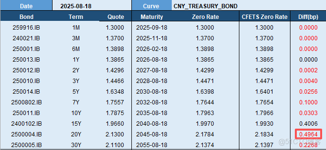
這裏，我們根據外匯交易中心（CFETS）2025 年 8 月份國債收益率曲線構建基準債券列表，選取 2025 年 8 月 18 日收盤數據，通過 Bootstrap 方法得到即期曲線（“Zero Rate” 列），並與 CFETS 即期曲線（“CFETS Zero Rate” 列）進行對比，發現最大誤差為期限 20Y 的 0.4964 個 bp，所有期限誤差均小於 0.5 個 bp。

基於 DolphinDB 構建收益率曲線與波動率曲面的最佳實踐_波動率曲面

2.2 Nelson-Siegel（NS）

Nelson-Siegel (NS) 模型最早由 Nelson 和 Siegel 於 1987 年提出，該模型適用於債券的利率期限結構分析。NS 模型中有四個參數，每個都有自身的經濟含義，不同參數值能描述不同情境下的利率曲線的變動情況（參考[1]）。

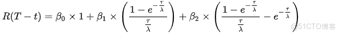
NS 模型假定了瞬時遠期利率的形式：

基於 DolphinDB 構建收益率曲線與波動率曲面的最佳實踐_波動率曲面_02

該模型有四個參數 β₀, β₁, β₂, λ，其中 τ=T-t 是到期年限，λ>0。

瞬時遠期利率 f(t, T) 裏面有三項：

第一項 β0 是當 τ 趨近無窮大時的遠期利率，因此 β0= f(∞)。
第二項是個單調函數，當 β1> 0 時遞減，當 β1 < 0 時遞增。
第三項是個非單調函數，可以產生凸起（hump）。

當 τ 趨近零時，第二項趨近於 β₁，第三項趨近於 0，因此 f(0) = β₀ + β₁。

對瞬時遠期利率求積分，可以得到即期利率的公式：（公式 1）

基於 DolphinDB 構建收益率曲線與波動率曲面的最佳實踐_波動率曲面_03

這樣容易看出：

β0 的因子載荷是常數，對於對所有期限利率的影響是相同的，因此 β0 可控制利率水平（level），它的變動會使得收益率曲線發生水平上下移動。
β1 的因子載荷是單調遞減，從1 很快的衰減到 0，這表明 β1 對短端利率的影響較大，因此 β1 可控制曲線斜率（slope），影響着利率曲線的斜率程度。
β2 的因子載荷先增後減，從 0 增到 1 再減到 0，這表明 β2 對利率曲線的短端和長端影響較弱，對中端的影響較大，因此 β2 控制曲線曲率（curvature）。
τ 是 β1 和 β2 的因子載荷的衰減速度，該值越大衰減越快。

NS模型構建即期曲線的過程首先是根據樣本券的到期收益率（YTM）報價，利用債券計算器（bondCalculator）得到債券全價（dirty），然後利用假設的即期曲線（公式 1）作為折現曲線對債券進行定價，得到理論價格 npv ，n 個樣本券可以得到 n 對 (dirty， npv)，最小化以下目標函數即可得到四個參數

基於 DolphinDB 構建收益率曲線與波動率曲面的最佳實踐_FICC_04

2.3 Nelson-Siegel-Svensson（NSS）

在 NS 基礎上，Svensson 在 1994 年做了改進，為了能多模擬一個 hump 形狀而增加了兩個參數。該模型下的瞬時遠期利率的形式為

基於 DolphinDB 構建收益率曲線與波動率曲面的最佳實踐_FICC_05

同時求積分我們可以得到其即期利率：

基於 DolphinDB 構建收益率曲線與波動率曲面的最佳實踐_波動率曲面_06

NSS 模型構建即期曲線的過程跟 NS 模型類似，只是即期曲線的函數解析式不同，暫不贅述。

2.4 示例

// 以2025年8月18日的國債收益率曲線構建為例
bond1 = {
    "productType": "Cash",
    "assetType": "Bond",
    "bondType": "DiscountBond",
    "instrumentId": "259916.IB",
    "start": 2025.03.13,
    "maturity": 2025.09.11,
    "issuePrice":  99.2070,
    "dayCountConvention": "ActualActualISDA"
}
bond2 = {
    "productType": "Cash",
    "assetType": "Bond",
    "bondType": "FixedRateBond",
    "instrumentId": "240021.IB",
    "start": 2024.10.25,
    "maturity": 2025.10.25,
    "coupon": 0.0133,
    "frequency": "Annual",
    "dayCountConvention": "ActualActualISDA"
}
bond3 = {
    "productType": "Cash",
    "assetType": "Bond",
    "bondType": "FixedRateBond",
    "instrumentId": "250001.IB",
    "start": 2025.01.15,
    "maturity": 2026.01.15,
    "coupon": 0.0116,
    "frequency": "Annual",
    "dayCountConvention": "ActualActualISDA"
}
bond4 = {
    "productType": "Cash",
    "assetType": "Bond",
    "bondType": "FixedRateBond",
    "instrumentId": "250013.IB",
    "start": 2025.07.25,
    "maturity": 2026.07.25,
    "coupon": 0.0133,
    "frequency": "Annual",
    "dayCountConvention": "ActualActualISDA"
}
bond5 = {
    "productType": "Cash",
    "assetType": "Bond",
    "bondType": "FixedRateBond",
    "instrumentId": "250012.IB",
    "start": 2025.06.15,
    "maturity": 2027.06.15,
    "coupon": 0.0138,
    "frequency": "Annual",
    "dayCountConvention": "ActualActualISDA"
}
bond6 = {
    "productType": "Cash",
    "assetType": "Bond",
    "bondType": "FixedRateBond",
    "instrumentId": "250010.IB",
    "start": 2025.05.25,
    "maturity": 2028.05.25,
    "coupon": 0.0146,
    "frequency": "Annual",
    "dayCountConvention": "ActualActualISDA"
}

referenceDate = 2025.08.18
bondsTmp = [bond1, bond2, bond3, bond4, bond5, bond6]
bonds = parseInstrument(bondsTmp)
/*
此案例對標的是外匯交易中心，使用標準期限，各個樣本券的剩餘期限(term)和報價(quote)都是虛擬出來的
https://www.chinamoney.com.cn/chinese/bkcurvclosedyhis/index.html
*/
terms = [1M, 3M, 6M, 1y, 2y, 3y]
quotes=[1.3000, 1.3700, 1.3898, 1.3865, 1.4296, 1.4466]/100
       
// method = "BoostStarp"
bootstrapCurve = bondYieldCurveBuilder(referenceDate, `CNY, bonds, terms, quotes, "ActualActualISDA", method='Bootstrap')
bootstrapCurveDict = extractMktData(bootstrapCurve)
print(bootstrapCurveDict)

// method = "NS"
nsCurve = bondYieldCurveBuilder(referenceDate, `CNY, bonds, terms, quotes, "ActualActualISDA", method='NS')
nsCurveDict = extractMktData(nsCurve)
print(nsCurveDict)

// method = "NSS"
nssCurve = bondYieldCurveBuilder(referenceDate, `CNY, bonds, terms, quotes, "ActualActualISDA", method='NSS')
nssCurveDict=extractMktData(nssCurve)
print(nssCurveDict)

3. 單貨幣利率互換曲線構建

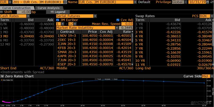
利率互換（IRS）是一種重要的金融衍生工具，它允許交易雙方在約定時期內，根據相同名義本金和不同利率計算方式，交換利息現金流。這通常涉及固定利率與浮動利率的交換，但不交換本金。利率互換定價需要用到利率互換曲線，我們這裏介紹單貨幣利率互換曲線構建，涉及到的金融工具包括：

存款利率 (Depo)：提供短期利率信息（如 1 天至 1 年）
遠期利率協議 (FRA)：提供短期到中期的遠期利率信息（如 3M-6M）
利率期貨 (Futures)：提供中短期的隱含遠期利率（如 3M-2Y）
利率互換 (Swaps)：提供中長期固定利率點（如 1Y-30Y）

基於 DolphinDB 構建收益率曲線與波動率曲面的最佳實踐_收益率曲線_07

3.1 Bootstrap

針對國內市場，我們選取的是 Depo 和 Swaps 作為構建工具，採用 Bootstrap 方法（算法請參考[2][3]）。這裏僅展示 CNY_FR_007 和 CNY_SHIBOR_3M 兩條曲線的構建結果。

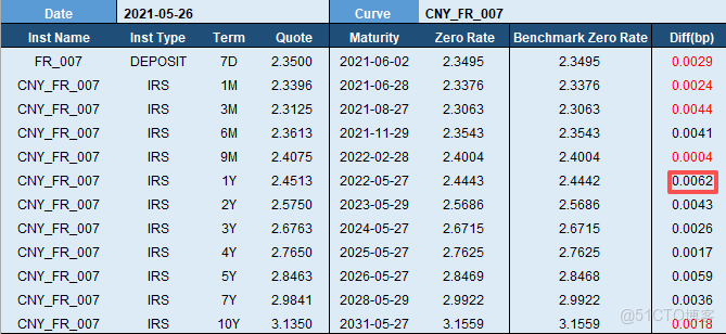
基於 DolphinDB 構建收益率曲線與波動率曲面的最佳實踐_波動率曲面_08

我們以2021年5月26日數據為例，根據 CNY_FR_007 各個期限交易的報價(“Quote”列)，利用 Bootstrap 方法，得到即期曲線 (“Zero Rate” 列) ，對比國內某大型機構的即期曲線（“Benchmark Zero Rate”），誤差幾乎為零。

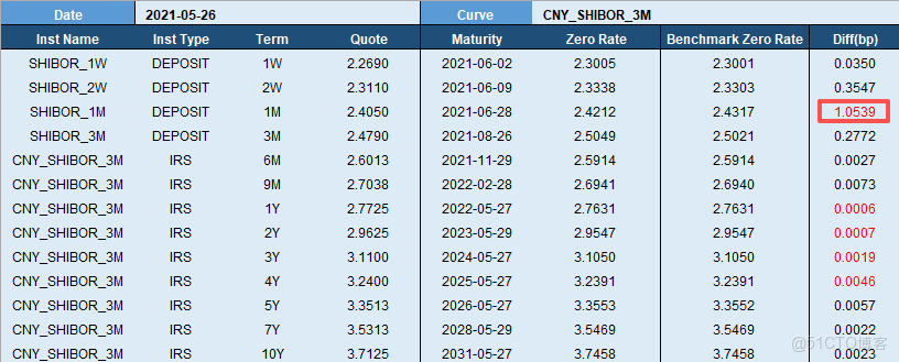
基於 DolphinDB 構建收益率曲線與波動率曲面的最佳實踐_FICC_09

我們以2021年5月26日數據為例，根據 CNY_SHIBOR_3M 各個期限交易的報價 (“Quote”列)，利用 Bootstrap 方法，得到即期曲線(“Zero Rate“列)，對比國內某大型機構的即期曲線（“Benchmark Zero Rate”），誤差最大為 1M 期的 1.0539bp，其餘期限誤差均小於 0.5bp。

3.2 示例

例1. 構建一條以人民幣計價、參考 FR_007 浮動利率的利率互換曲線。

referenceDate = 2021.05.26
currency = "CNY"
terms = [7d, 1M, 3M, 6M, 9M, 1y, 2y, 3y, 4y, 5y, 7y, 10y]
instNames = take("CNY_FR_007", size(terms))
instNames[0] = "FR_007"
instTypes = take("IrVanillaSwap", size(terms))
instTypes[0] = "Deposit"
quotes = [2.3500, 2.3396, 2.3125, 2.3613, 2.4075, 2.4513, 2.5750, 2.6763, 2.7650, 2.8463, 2.9841, 3.1350]\100
dayCountConvention = "Actual365"
curve = irSingleCurrencyCurveBuilder(referenceDate, currency, instNames, instTypes, terms, quotes, dayCountConvention, curveName="CNY_FR_007")
curveDict = extractMktData(curve)
print(curveDict)

例2. 構建一條以人民幣計價、參考 SHIBOR_3M 浮動利率的利率互換曲線。

referenceDate = 2021.05.26
currency = "CNY"
terms = [1w, 2w, 1M, 3M, 6M, 9M, 1y, 2y, 3y, 4y, 5y, 7y, 10y]
instNames = take("CNY_SHIBOR_3M", size(terms))
instNames[0] = "SHIBOR_1W"
instNames[1] = "SHIBOR_2W"
instNames[2] = "SHIBOR_1M"
instNames[3] = "SHIBOR_3M"
instTypes = take("IrVanillaSwap", size(terms))
instTypes[0] = "Deposit"
instTypes[1] = "Deposit"
instTypes[2] = "Deposit"
instTypes[3] = "Deposit"
quotes = [2.269, 2.311, 2.405, 2.479, 2.6013, 2.7038,2.7725,
          2.9625, 3.11, 3.24, 3.3513, 3.5313, 3.7125]/100
dayCountConvention = "Actual365"
curve = irSingleCurrencyCurveBuilder(referenceDate, currency, instNames, instTypes, terms, quotes, dayCountConvention)
curveDict = extractMktData(curve)
print(curveDict)

4. 外幣隱含利率曲線構建

在外匯產品的定價中，需要輸入兩種貨幣的即期曲線來分別表示各自的資金成本，所以構建外幣的隱含利率曲線也是很重要的。通常情況下，構建外幣隱含利率曲線的金融工具有：

外匯掉期 (FxSwap)：提供短期利率信息
貨幣交叉互換 (CrossCurrencySwap)：提供中期到遠期期的利率信息

4.1 Bootstrap

對於國內市場，我們全部採用 FxSwap 和外匯即期報價，通過利率平價公式，推導出外幣的隱含利率曲線。根據遠期匯率公式（以連續複利為例）：

基於 DolphinDB 構建收益率曲線與波動率曲面的最佳實踐_FICC_10

基於 DolphinDB 構建收益率曲線與波動率曲面的最佳實踐_收益率曲線_11

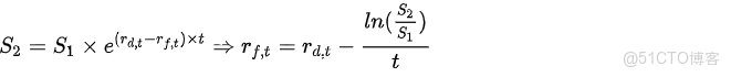
其中 S₁ 為近端（即期）匯率，S₂ 為遠端匯率，t 為掉期的期限，SwapPoint_t 為外匯掉期的報價，r_d,t 為對應期限 t 的本幣零息利率。根據上式即可推導出期限 t 對應的外幣的零息利率 r_f,t 。

這裏展示一條美元隱含收益率曲線（USD_USDCNY_FX）的構建結果：

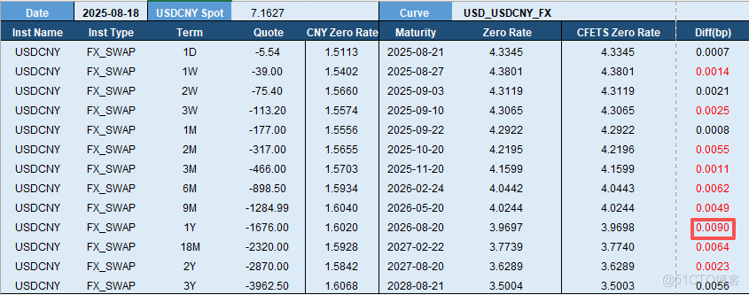
基於 DolphinDB 構建收益率曲線與波動率曲面的最佳實踐_FICC_12

根據外匯交易中心提供的2025年8月18日 USDCNY 外匯掉期報價(“Quote” 列)、即期匯率和人民幣即期利率曲線（“CNY Zero Rate”列），利用利率平價公式，得到美元即期曲線（“Zero Rate” 列），對比外匯交易中心的美元即期曲線（“CFETS Zero Rate”），誤差幾乎為零。

4.2 示例

// 以2025年8月18日的USDCNY美元隱含收益率曲線構建為例
refDate = 2025.08.18
spotDate1 = temporalAdd(refDate, 2, "XNYS")    //美元的即期日，其中“XNYS”為美國交易日曆   
spotDate2 = temporalAdd(refDate, 2, "CFET")   //人民幣的即期日，其中“XNYS”為中國交易日曆   
spotDate = max(spotDate1, spotDate2)
instNames = take("USDCNY", 13)
instTypes = take("FxSwap", 13)
terms = ["1d", "1w", "2w", "3w", "1M", "2M", "3M", "6M", "9M", "1y", "18M", "2y", "3y"]
curveDates = array(DATE)
// 計算每個外匯掉期報價到期日，作為曲線的時間軸
for(term in terms){
    dur = duration(term)
    d1 = transFreq(temporalAdd(spotDate, dur), "XNYS", "right", "right")
    d2 = transFreq(temporalAdd(spotDate, dur), "CFET", "right", "right")
    curveDates.append!(max(d1, d2))
 }
quotes = [-5.54, -39.00, -75.40, -113.20, -177.00, -317.00, -466.00, -898.50, 
         -1284.99, -1676.00, -2320.00, -2870.00, -3962.50] \ 10000  // fx swap points

curve = {
    "mktDataType": "Curve",
    "curveType": "IrYieldCurve",
    "referenceDate": refDate,
    "currency": "CNY",
    "dayCountConvention": "Actual365",
    "compounding": "Continuous",
    "interpMethod": "Linear",
    "extrapMethod": "Flat",
    "dates": curveDates,
    "values": [1.5113, 1.5402, 1.5660, 1.5574, 1.5556, 1.5655, 1.5703, 
               1.5934, 1.6040, 1.6020, 1.5928, 1.5842, 1.6068] \ 100,
    "settlement": spotDate
}

cnyShibor3m = parseMktData(curve)

spot = 7.1627
curve = irCrossCurrencyCurveBuilder(refDate, "USD", instNames, instTypes, terms, quotes, "USDCNY", spot, "Actual365", cnyShibor3m, "Continuous")
curveDict = extractMktData(curve)
for(i in 0..(size(quotes)-1) ){
    print(curveDict["values"][i]*100)
}

5. 外匯期權波動率曲面構建

外匯期權定價需要用到波動率，而對於單個期權而言，其波動率需要按照自身的執行價和剩餘期限從波動率曲面中插值出來。不同於其他資產對應期權的 strike-vol 報價，外匯期權報價採用 delta-vol 的形式，所以曲面構建的第一步就是 delta 轉 strike，轉換過程如下：

//Step1：計算出單個期權對應的vol
sigma_25c = sigma_atm + bf_25 + 0.5 * rr_25   //delta = 0.25的vol
sigma_25p = sigma_atm + bf_25 - 0.5 * rr_25   //delta =-0.25的vol
sigma_10c = sigma_atm + bf_10 + 0.5 * rr_10   //delta = 0.10的vol
sigma_10p = sigma_atm + bf_10 - 0.5 * rr_10   //delta =-0.10的vol
/*
其中
sigma_atm：平值期權報價
bf_25：delta=0.25的碟式（Butterfly）期權報價  
rr_25：delta=0.25的風險逆轉（Risk Reversal）期權報價  
bf_10：delta=0.10的碟式（Butterfly）期權報價  
rr_10：delta=0.10的風險逆轉（Risk Reversal）期權報價 
*/

//Step2：根據Black-Scholes計算delta的公式反堆strike，這裏不展開，請參考文獻[5]

得到 strike-vol（smile）離散點之後，就可以根據以下模型構建波動率微笑了。由於線性插值（Linear）和三次樣條插值（CubicSpile）構建波動率微笑比較簡單，這裏不展開，重點介紹 SVI 和 SABR 模型。

5.1 SVI（Stochastic Volatility Inspired）

SVI 模型由 Jim Gatheral 提出，通過總方差建模隱含波動率微笑：（公式 2）

基於 DolphinDB 構建收益率曲線與波動率曲面的最佳實踐_收益率曲線_13

其中：

ω(k)：總方差，定義 ω(k)=σ2imp×T，σ2imp 為隱含波動率，T 為到期時間
k：對數 moneyness，k=ln(K/F)，K 為行權價格，F 為遠期匯率
a：最小總方差，控制總方差的基準水平
b：控制總方差的傾斜程度
ρ：控制微笑的對稱性（ρ∈[-1,1]），通常為負值
m：對數 moneyness 的中心位置
σ：控制微笑的寬帶

公式 2 中的左邊可以根據上一節 strike-vol 得到，strike 就是 k=ln(K/F) 的計算公式中的 K（F 可以根據遠期匯率公式計算）， vol 就是 σ_imp 。定義目標函數

基於 DolphinDB 構建收益率曲線與波動率曲面的最佳實踐_波動率曲面_14

可以採用 Levenberg-Marquardt 等算法最小化目標函數，求出五個參數，即可得到整個 smile 曲線上任意 strike 對應的 vol。

5.2 SABR（Stochastic Alpha Beta Rho）

SABR 模型的隱含波動率近似公式為：

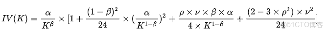
基於 DolphinDB 構建收益率曲線與波動率曲面的最佳實踐_FICC_15

其中：

IV(K)：行權價格 K 對應的隱含波動率
α：初始波動率，控制波動率水平
β：控制波動率對標的價格的敏感性，取值範圍為 [0,1]
ρ：標的資產價格與波動率之間的相關性
υ：波動率的波動率（vol-of-vol）
K ：行權價格
F ：遠期匯率
T ：到期時間

定義目標函數

基於 DolphinDB 構建收益率曲線與波動率曲面的最佳實踐_收益率曲線_16

採用 Levenberg-Marquardt 等算法最小化目標函數，求出四個參數，即可得到整個 smile 曲線上任意 strike 對應的 vol。

5.3 示例

基於 DolphinDB 構建收益率曲線與波動率曲面的最佳實踐_收益率曲線_17

基於 DolphinDB 構建收益率曲線與波動率曲面的最佳實踐_FICC_18

基於 DolphinDB 構建收益率曲線與波動率曲面的最佳實踐_FICC_19

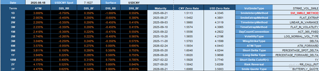
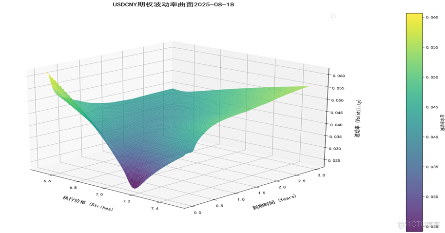
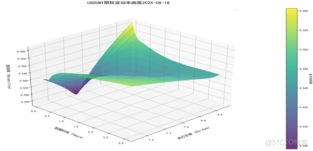
以外匯交易中心 2025 年 8 月 18 日數據為例，選取 USDCNY 外匯期權 delta 報價矩陣為參數，SVI 模型擬合波動率微笑，得到了外匯波動率曲面，該曲面可用作外匯期權的定價。

refDate = 2025.08.18
ccyPair = "USDCNY"
quoteTerms = ['1d', '1w', '2w', '3w', '1M', '2M', '3M', '6M', '9M', '1y', '18M', '2y', '3y']
quoteNames = ["ATM", "D25_RR", "D25_BF", "D10_RR", "D10_BF"]
quotes = [0.030000, -0.007500, 0.003500, -0.010000, 0.005500, 
          0.020833, -0.004500, 0.002000, -0.006000, 0.003800, 
          0.022000, -0.003500, 0.002000, -0.004500, 0.004100, 
          0.022350, -0.003500, 0.002000, -0.004500, 0.004150, 
          0.024178, -0.003000, 0.002200, -0.004750, 0.005500, 
          0.027484, -0.002650, 0.002220, -0.004000, 0.005650, 
          0.030479, -0.002500, 0.002400, -0.003500, 0.005750, 
          0.035752, -0.000500, 0.002750,  0.000000, 0.006950, 
          0.038108,  0.001000, 0.002800,  0.003000, 0.007550, 
          0.039492,  0.002250, 0.002950,  0.005000, 0.007550, 
          0.040500,  0.004000, 0.003100,  0.007000, 0.007850, 
          0.041750,  0.005250, 0.003350,  0.008000, 0.008400, 
          0.044750,  0.006250, 0.003400,  0.009000, 0.008550]
quotes = reshape(quotes, size(quoteNames):size(quoteTerms)).transpose()
spot = 7.1627
curveDates = [2025.08.21, 2025.08.27, 2025.09.03, 2025.09.10, 2025.09.22, 2025.10.20,
  2025.11.20, 2026.02.24,2026.05.20, 2026.08.20, 2027.02.22, 2027.08.20, 2028.08.21]
domesticCurveInfo = {
    "mktDataType": "Curve",
    "curveType": "IrYieldCurve",
    "referenceDate": refDate,
    "currency": "CNY",
    "dayCountConvention": "Actual365",
    "compounding": "Continuous",  
    "interpMethod": "Linear",
    "extrapMethod": "Flat",
    "frequency": "Annual",
    "dates": curveDates,
    "values":[1.5113, 1.5402, 1.5660, 1.5574, 1.5556, 1.5655, 1.5703, 
              1.5934, 1.6040, 1.6020, 1.5928, 1.5842, 1.6068]/100
}
foreignCurveInfo = {
    "mktDataType": "Curve",
    "curveType": "IrYieldCurve",
    "referenceDate": refDate,
    "currency": "USD",
    "dayCountConvention": "Actual365",
    "compounding": "Continuous",  
    "interpMethod": "Linear",
    "extrapMethod": "Flat",
    "frequency": "Annual",
    "dates": curveDates,
    "values":[4.3345, 4.3801, 4.3119, 4.3065, 4.2922, 4.2196, 4.1599, 
              4.0443, 4.0244, 3.9698, 3.7740, 3.6289, 3.5003]/100
}
domesticCurve = parseMktData(domesticCurveInfo)
foreignCurve = parseMktData(foreignCurveInfo)
surf = fxVolatilitySurfaceBuilder(refDate, ccyPair, quoteNames, quoteTerms, quotes, spot, domesticCurve, foreignCurve)
surfDict = extractMktData(surf)
print(surfDict)

6. 工具函數

6.1 curvePredict

構建好曲線之後，我們可以通過 curvePredict 函數獲取任意時間的曲線值。

curveDict = {
    "mktDataType": "Curve",
    "curveType": "IrYieldCurve",
    "referenceDate": 2025.08.18,
    "currency": "CNY",
    "dayCountConvention": "ActualActualISDA",
    "compounding": "Continuous",  
    "interpMethod": "Linear",
    "extrapMethod": "Flat",
    "frequency": "Annual",
    "dates": [2025.08.21, 2025.08.27, 2025.09.03, 2025.09.10, 2025.09.22, 2025.10.20,
     2025.11.20, 2026.02.24, 2026.05.20, 2026.08.20, 2027.02.22,2027.08.20, 2028.08.21],
    "values":[1.5113, 1.5402, 1.5660, 1.5574, 1.5556, 1.5655, 1.5703, 
              1.5934, 1.6040, 1.6020, 1.5928, 1.5842, 1.6068]/100
}

curve = parseMktData(curveDict)
curvePredict(curve, 2025.10.18)
// output: 0.0156
curvePredict(curve, 1.0)
// output: 0.0160
curvePredict(curve, [2025.10.18, 2026.10.18])
// output: [0.0156,0.0159]
curvePredict(curve, [1.0, 2.0])
// output: [0.0160,0.0158]

6.2 optionVolPredict

波動率曲面是一個三維曲面，我們可以通過 optionVolPredict 獲取指定時間和執行價時曲面上的波動率。

refDate = 2025.08.18
ccyPair = "USDCNY"
quoteTerms = ['1d', '1w', '2w', '3w', '1M', '2M', '3M', '6M', '9M', '1y', '18M', '2y', '3y']
quoteNames = ["ATM", "D25_RR", "D25_BF", "D10_RR", "D10_BF"]
quotes = [0.030000, -0.007500, 0.003500, -0.010000, 0.005500, 
          0.020833, -0.004500, 0.002000, -0.006000, 0.003800, 
          0.022000, -0.003500, 0.002000, -0.004500, 0.004100, 
          0.022350, -0.003500, 0.002000, -0.004500, 0.004150, 
          0.024178, -0.003000, 0.002200, -0.004750, 0.005500, 
          0.027484, -0.002650, 0.002220, -0.004000, 0.005650, 
          0.030479, -0.002500, 0.002400, -0.003500, 0.005750, 
          0.035752, -0.000500, 0.002750,  0.000000, 0.006950, 
          0.038108,  0.001000, 0.002800,  0.003000, 0.007550, 
          0.039492,  0.002250, 0.002950,  0.005000, 0.007550, 
          0.040500,  0.004000, 0.003100,  0.007000, 0.007850, 
          0.041750,  0.005250, 0.003350,  0.008000, 0.008400, 
          0.044750,  0.006250, 0.003400,  0.009000, 0.008550]

quotes = reshape(quotes, size(quoteNames):size(quoteTerms)).transpose()

spot = 7.1627
curveDates = [2025.08.21, 2025.08.27, 2025.09.03, 2025.09.10, 2025.09.22, 2025.10.20,
  2025.11.20, 2026.02.24, 2026.05.20, 2026.08.20, 2027.02.22, 2027.08.20, 2028.08.21]

domesticCurveInfo = {
    "mktDataType": "Curve",
    "curveType": "IrYieldCurve",
    "referenceDate": refDate,
    "currency": "CNY",
    "dayCountConvention": "Actual365",
    "compounding": "Continuous",  
    "interpMethod": "Linear",
    "extrapMethod": "Flat",
    "frequency": "Annual",
    "dates": curveDates,
    "values":[1.5113, 1.5402, 1.5660, 1.5574, 1.5556, 1.5655, 1.5703, 
              1.5934, 1.6040, 1.6020, 1.5928, 1.5842, 1.6068]/100
}
foreignCurveInfo = {
    "mktDataType": "Curve",
    "curveType": "IrYieldCurve",
    "referenceDate": refDate,
    "currency": "USD",
    "dayCountConvention": "Actual365",
    "compounding": "Continuous",  
    "interpMethod": "Linear",
    "extrapMethod": "Flat",
    "frequency": "Annual",
    "dates": curveDates,
    "values":[4.3345, 4.3801, 4.3119, 4.3065, 4.2922, 4.2196, 4.1599, 
              4.0443, 4.0244, 3.9698, 3.7740, 3.6289, 3.5003]/100
}

domesticCurve = parseMktData(domesticCurveInfo)
foreignCurve = parseMktData(foreignCurveInfo)

surf = fxVolatilitySurfaceBuilder(refDate, ccyPair, quoteNames, quoteTerms, quotes, spot, domesticCurve, foreignCurve)

optionVolPredict(surf, 2025.10.18, 7)
/* output:
           7                
           -----------------
2025.10.18|0.035427722673281
*/
optionVolPredict(surf, 2025.10.18, [7.1,7.2])
/* output:
           7.1               7.2
           ----------------- -----------------
2025.10.18|0.029466799513362 0.029268084254983
*/
optionVolPredict(surf, [2025.10.18, 2026.10.18], 7)
/* output:
           7                
           -----------------
2025.10.18|0.035427722673281
2026.10.18|0.040453528763062
*/
optionVolPredict(surf, [2025.10.18, 2026.10.18], [7.1, 7.2])
/* output:
           7.1               7.2
           ----------------- -----------------
2025.10.18|0.029466799513362 0.029268084254983
2026.10.18|0.042188693924168 0.044408563755123
*/

7. 總結與展望

本教程展示了部分利率曲線和外匯期權波動率曲面的構建理論和方法，並用 DolphinDB 內置函數逐一進行了使用説明，結果和相關基準進行了對比，同時提供了工具函數方便用户使用。

後續我們會在兩個方面不斷迭代與更新：

增加更多的曲線/曲面構建函數，比如商品遠期曲線、CDS 信用利差曲線、商品期權波動率曲面等
同一個函數增加更多的標的品種，比如單貨幣利率互換曲線構建函數（irSingleCurrencyCurveBuilder）目前僅支持 CNY_FR_007 和 CNY_SHIBOR_3M，後續會增加 USD_SOFR / EUR_ESTR 等曲線

收益率曲線和波動率曲面構建是金融工程的核心功能，這些中間市場數據不僅是定價和風控的前提，也為眾多量化策略（參考[6]）提供了幫助。隨着中國金融市場的不斷崛起，我們會緊跟市場，提供更多的金融工程函數來服務客户，敬請期待！

參考

[1] 債券收益率曲線構建

[2]『曲線構建系列 1』單曲線方法

[3] F. Ametrano and M. Bianchetti. Everything you always wanted to know about Multiple In terest Rate Curve Bootstrapping but were afraid to ask (April 2, 2013). Available at SSRN: Everything You Always Wanted to Know About Multiple Interest Rate Curve Bootstrapping but Were Afraid to Ask or Everything You Always Wanted to Know About Multiple Interest Rate Curve Bootstrapping but Were Afraid to Ask , 2013.

[4] Reiswich, D., & Wystup, U. (2010). FX Volatility Smile Construction. CPQF Working Paper Series, No. 20. Frankfurt School of Finance & Management.

[5] Clark, I. J. (2011). Foreign exchange option pricing: A practitioner's guide. Chichester, West Sussex, PO19 8SQ, United Kingdom: John Wiley & Sons Ltd.

[6] 徐寒飛. 債券量化研究系列專題之二：收益率曲線交易[R]. 廣州: 廣發證券股份有限公司, 2013-01-08.

附錄

curve_volsurf_builder.dos

u_15022783 博客

u_15022783 博客

博客 / 詳情