

1. 常規情況
基礎知識:
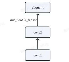
- 考慮到模型輸出位置量化損失對模型精度的影響較大,工具鏈推薦模型以 linear/conv 結尾,此時支持高精度 int32 輸出(在 quantized.onnx 中,轉定點為 int32,在前面 calib+qat 階段都是 float32),這幾乎可以做到無損。
- 征程 6 工具鏈量化 setter 模板支持自動設置高精度輸出,前提是 conv 輸出直接 接 dequant,不作為其他 node 的輸入。
輸出位置結構示意圖:
全流程代碼如下:
import torch
from horizon_plugin_pytorch import set_march, March
set_march(March.NASH_M)
from horizon_plugin_pytorch.quantization import prepare, set_fake_quantize, FakeQuantState
from horizon_plugin_pytorch.quantization import QuantStub
from horizon_plugin_pytorch.quantization.hbdk4 import export
from horizon_plugin_pytorch.quantization.qconfig_template import (
    calibration_8bit_weight_16bit_act_qconfig_setter,
    qat_8bit_weight_16bit_fixed_act_qconfig_setter,
    default_calibration_qconfig_setter,
    ModuleNameQconfigSetter
)

from horizon_plugin_pytorch.quantization.qconfig import get_qconfig, MSEObserver, MinMaxObserver
from horizon_plugin_pytorch.dtype import qint8, qint16
from torch.quantization import DeQuantStub
import torch.nn as nn
from horizon_plugin_pytorch.quantization import hbdk4 as hb4
from hbdk4.compiler import convert, save, hbm_perf, visualize, compile

import torch
import torch.nn as nn

# 定義網絡結構
class SmallModel(nn.Module):
    def __init__(self):
        super(SmallModel, self).__init__()
        # 第一個 Linear: 輸入 [2, 100, 256] -> 輸出 [2, 100, 256]
        self.linear1 = nn.Linear(256, 256)
        self.layernorm = nn.LayerNorm(256)  # 對最後一維進行歸一化
        self.relu = nn.ReLU()
        # 第二個 Linear: 輸入 [2, 100, 256] -> 輸出 [2, 100, 60]
        self.linear2 = nn.Linear(256, 60)
        # 第三個 Linear: 輸入 [2, 100, 60] -> 輸出 [2, 100, 60]
        self.linear3 = nn.Linear(60, 60)
        self.quant = QuantStub()
        self.dequant = DeQuantStub()

    def forward(self, x):
        x = self.quant(x)
        # 第一個 Linear
        x = self.linear1(x)  # [2, 100, 256]
        x = self.layernorm(x)  # [2, 100, 256]
        x = self.relu(x)  # [2, 100, 256]
        # 第二個 Linear
        y = self.linear2(x)  # [2, 100, 60]
        # 第三個 Linear
        z = self.linear3(y)
        z = self.dequant(z)
        return z

# 設置隨機種子,保證每次生成的數據相同
torch.manual_seed(42)
example_input = torch.randn(2, 100, 256)
model = SmallModel()

# 前向傳播
output_x = model(example_input)
print("輸入形狀:", example_input.shape)
print("輸出形狀:", output_x.shape)

# A global march indicating the target hardware version must be setted before prepare qat.
set_march(March.NASH_M)

calib_model = prepare(model.eval(), example_input,
                      qconfig_setter=(
                          default_calibration_qconfig_setter,
                          ),
                      )

calib_model.eval()
set_fake_quantize(calib_model, FakeQuantState.CALIBRATION)
calib_model(example_input)

calib_model.eval()
set_fake_quantize(calib_model, FakeQuantState.VALIDATION)
calib_out_x = calib_model(example_input)
print("calib輸出shape:", calib_out_x.shape)

qat_bc = export(calib_model, example_input)
# save(qat_bc, "qat.bc")
# visualize(qat_bc, "qat.onnx")
hb_quantized_model = convert(qat_bc, March.NASH_M)
# save(hb_quantized_model,"quantized.bc")
visualize(hb_quantized_model, "quantized_single.onnx")
查看 quantized.onnx,可以看到最後一個 conv 確實是 int32 高精度輸出
2. 輸出又輸入
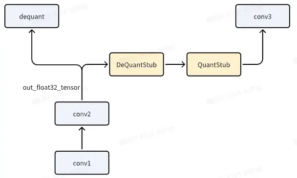
如果 conv1,既作為模型輸出,又作為後續 conv2 的輸入,此時應該怎麼辦?
關鍵代碼如下:
def forward(self, x):
        x = self.quant(x)
        # 第一個 Linear
        x = self.linear1(x)  # [2, 100, 256]
        x = self.layernorm(x)  # [2, 100, 256]
        x = self.relu(x)  # [2, 100, 256]
        # 第二個 Linear
        y = self.linear2(x)  # [2, 100, 60]
        y_out = self.dequant(y)
        y = self.quant_out(y_out)
        # y = self.quant_out(y)

        # 第三個 Linear
        z = self.linear3(y)
        z = self.dequant(z)
        return x, y_out
注意,y\_out = self.dequant(y)是必須要添加的,否則無法實現該效果。
全流程代碼如下:
import torch
from horizon_plugin_pytorch import set_march, March
set_march(March.NASH_M)
from horizon_plugin_pytorch.quantization import prepare, set_fake_quantize, FakeQuantState
from horizon_plugin_pytorch.quantization import QuantStub
from horizon_plugin_pytorch.quantization.hbdk4 import export
from horizon_plugin_pytorch.quantization.qconfig_template import (
calibration_8bit_weight_16bit_act_qconfig_setter,
qat_8bit_weight_16bit_fixed_act_qconfig_setter,
default_calibration_qconfig_setter,
ModuleNameQconfigSetter
)
from horizon_plugin_pytorch.quantization.qconfig import get_qconfig, MSEObserver, MinMaxObserver
from horizon_plugin_pytorch.dtype import qint8, qint16
from torch.quantization import DeQuantStub
import torch.nn as nn
from horizon_plugin_pytorch.quantization import hbdk4 as hb4
from hbdk4.compiler import convert, save, hbm_perf, visualize, compile
import torch
import torch.nn as nn
# 定義網絡結構
class SmallModel(nn.Module):
def __init__(self):
super(SmallModel, self).__init__()
# 第一個 Linear: 輸入 [2, 100, 256] -> 輸出 [2, 100, 256]
self.linear1 = nn.Linear(256, 256)
self.layernorm = nn.LayerNorm(256) # 對最後一維進行歸一化
self.relu = nn.ReLU()
# 第二個 Linear: 輸入 [2, 100, 256] -> 輸出 [2, 100, 60]
self.linear2 = nn.Linear(256, 60)
# 第三個 Linear: 輸入 [2, 100, 60] -> 輸出 [2, 100, 60]
self.linear3 = nn.Linear(60, 60)
self.quant = QuantStub()
self.quant_out = QuantStub()
self.dequant = DeQuantStub()
def forward(self, x):
x = self.quant(x)
# 第一個 Linear
x = self.linear1(x) # [2, 100, 256]
x = self.layernorm(x) # [2, 100, 256]
x = self.relu(x) # [2, 100, 256]
# 第二個 Linear
y = self.linear2(x) # [2, 100, 60]
y_out = self.dequant(y)
y = self.quant_out(y_out)
# 第三個 Linear
z = self.linear3(y)
z = self.dequant(z)
return z, y_out
# 設置隨機種子,保證每次生成的數據相同
torch.manual_seed(42)
example_input = torch.randn(2, 100, 256)
model = SmallModel()
# 前向傳播
output_x, output_y = model(example_input)
print("輸入形狀:", example_input.shape)
print("輸出形狀:", output_x.shape, output_y.shape)
# A global march indicating the target hardware version must be setted before prepare qat.
set_march(March.NASH_M)
calib_model = prepare(model.eval(), example_input,
qconfig_setter=(
default_calibration_qconfig_setter,
),
)
calib_model.eval()
set_fake_quantize(calib_model, FakeQuantState.CALIBRATION)
calib_model(example_input)
calib_model.eval()
set_fake_quantize(calib_model, FakeQuantState.VALIDATION)
calib_out_x, calib_out_y= calib_model(example_input)
print("calib輸出shape:", calib_out_x.shape)
qat_bc = export(calib_model, example_input)
# save(qat_bc, "qat.bc")
# visualize(qat_bc, "qat.onnx")
hb_quantized_model = convert(qat_bc, March.NASH_M)
# save(hb_quantized_model,"quantized.bc")
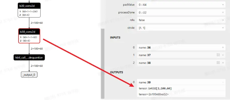
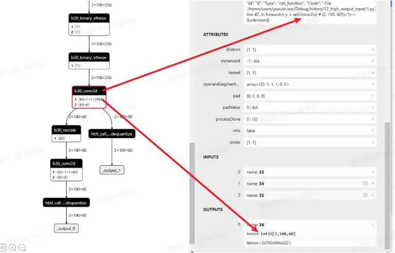
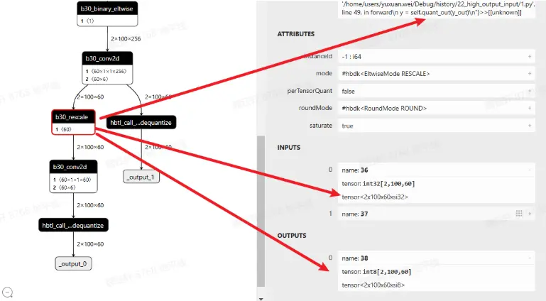
visualize(hb_quantized_model, "quantized.onnx")查看 quantized.onnx,linear2 符合預期,確實是 int32 高精度輸出。
新加入的 dequant 與 quant 會變成 rescale
以上是征程 6EM 的默認做法,如果使用的是征程 6PH,conv like 算子輸出直接就是 float32,在既作為輸出,又作為下一階段輸入時,會存在 vpu 的 quantize(float32->int16/int8),如下圖所示
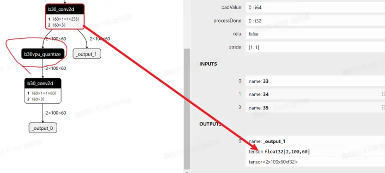
如果想依舊沿用征程 6EM 的方式,可進行如下配置:
qat_bc._integer_conv = True
hb_quantized_model = convert(qat_bc, "nash-h")
具體選擇哪種方式可實測 latency(建議考慮將模型 conv like 算子 c++ 反量化的耗時減少也加進去對比)