對於神經網絡來説，我們已經習慣了層狀網絡的思維：數據進來，經過第一層，然後第二層，第三層，最後輸出結果。這個過程很像流水線，每一步都是離散的。

但是現實世界的變化是連續的，比如燒開水，誰的温度不是從30度直接跳到40度，而是平滑的上生。球從山坡滾下來速度也是漸漸加快的。這些現象背後都有連續的規律在支配。

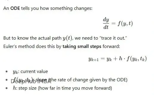
微分方程就是描述這種連續變化的語言。它不關心某個時刻的具體數值，而是告訴你"變化的速度"。比如説，温度下降得有多快？球加速得有多猛？

Neural ODE的想法很直接：自然界是連續的，神經網絡要是離散的？與其讓數據在固定的層之間跳躍，不如讓它在時間維度上平滑地演化。

微分方程的概念

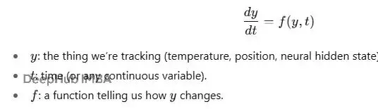
微分方程其實就是描述變化的規則。

最簡單的例子是咖啡冷卻。剛泡好的咖啡温度高，冷卻很快；温度接近室温時，冷卻就變慢了。這個現象背後的規律是：冷卻速度和温度差成正比。

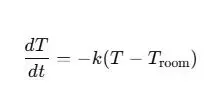
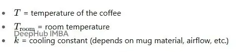
比如説：90°C的咖啡在22°C房間裏，温差68度，冷卻很快；30°C的咖啡在同樣環境裏，温差只有8度，冷卻就慢得多。這就是為什麼咖啡從燙嘴快速降到能喝的温度，然後就一直保持温熱狀態。

這不只是個咖啡的故事，它展示了動態系統的核心特徵：當前狀態決定了變化的方向和速度。ODE捕捉的正是這種連續演化的規律。

 # 1) 咖啡冷卻曲線（指數衰減到室温）  

import numpy as np  
import matplotlib.pyplot as plt  

# 咖啡冷卻曲線 ----------  
# 冷卻模型參數：dT/dt = -k (T - T_room)  
T0 = 90.0          # 初始温度 (°C)  
T_room = 22.0      # 室温 (°C)  
k = 0.35           # 冷卻常數 (1/min)  
t = np.linspace(0, 20, 300)  # 分鐘  

T = T_room + (T0 - T_room) * np.exp(-k * t)  

plt.figure(figsize=(7, 5))  
plt.plot(t, T, linewidth=2)  
plt.title("Coffee Cooling: An ODE in Action")  
plt.xlabel("Time (minutes)")  
plt.ylabel("Temperature (°C)")  
plt.grid(True, alpha=0.3)  
coffee_path = "/data/coffee_cooling_curve.png"  
plt.tight_layout()  
plt.savefig(coffee_path, dpi=200, bbox_inches="tight")  
 plt.show()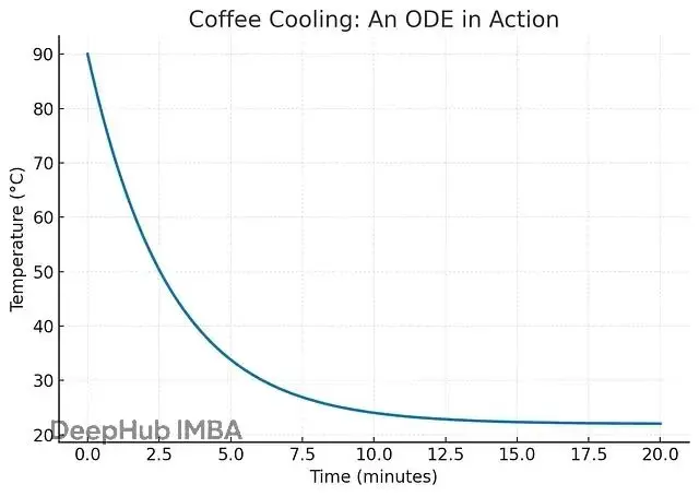

另一個例子是球滾下山坡。球剛開始幾乎不動，但重力會讓它加速。滾得越快摩擦阻力越大，最終速度會趨於穩定。整個過程可以用一個ODE來描述：

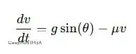
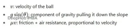
這個方程抓住了兩個關鍵力量：重力讓球加速、摩擦讓球減速，速度的變化取決於這兩個力的平衡。從數學上看，這個簡單的方程能完整地描述球從靜止到終端速度的整個過程。

 
    import numpy as np  
    import matplotlib.pyplot as plt  
      
    # ---------------- 參數 ----------------  
    g = 9.81           # 重力 (m/s^2)  
    theta_deg = 15.0   # 坡度角（度）  
    theta = np.deg2rad(theta_deg)  
    mu = 0.4           # 線性阻力系數 (1/s)  
      
    v0 = 0.0           # 初始速度 (m/s)  
    x0 = 0.0           # 初始位置 (m)  
    t_end = 12.0       # 總仿真時間 (s)  
    n_steps = 1200     # 積分步數  

# ---------------- 時間網格 ----------------  
t = np.linspace(0.0, t_end, n_steps)  

# ---------------- 向量場 ----------------  
def f(y, ti):  
    x, v = y  
    dv = g*np.sin(theta) - mu*v  
    dx = v  
    return np.array([dx, dv], dtype=float)  

# ---------------- RK4積分器 ----------------  
def rk4(f, y0, t):  
    y = np.zeros((len(t), len(y0)), dtype=float)  
    y[0] = y0  
    for i in range(1, len(t)):  
        h = t[i] - t[i-1]  
        ti = t[i-1]  
        yi = y[i-1]  
        k1 = f(yi, ti)  
        k2 = f(yi + 0.5*h*k1, ti + 0.5*h)  
        k3 = f(yi + 0.5*h*k2, ti + 0.5*h)  
        k4 = f(yi + h*k3, ti + h)  
        y[i] = yi + (h/6.0)*(k1 + 2*k2 + 2*k3 + k4)  
    return y  

# ---------------- 數值積分 ----------------  
y0 = np.array([x0, v0])  
traj = rk4(f, y0, t)  
x_num = traj[:, 0]  
v_num = traj[:, 1]  

# ---------------- 解析解 ----------------  
v_inf = (g*np.sin(theta)) / mu if mu != 0 else np.inf  
v_ana = v_inf + (v0 - v_inf) * np.exp(-mu * t)  
x_ana = x0 + v_inf*t + ((v0 - v_inf)/mu) * (1.0 - np.exp(-mu*t))  

# ---------------- 圖1：速度 ----------------  
plt.figure(figsize=(8.5, 5))  
plt.plot(t, v_num, linewidth=2, label="Velocity — RK4 (numeric)")  
plt.plot(t, v_ana, linewidth=2, linestyle="--", label="Velocity — analytic")  
plt.axhline(v_inf, linestyle=":", label=f"Terminal velocity = {v_inf:.2f} m/s")  
plt.title(f"Ball Rolling Downhill — Velocity vs Time (θ={theta_deg:.1f}°, μ={mu})")  
plt.xlabel("Time (s)")  
plt.ylabel("Velocity (m/s)")  
plt.grid(True, alpha=0.3)  
plt.legend(frameon=False)  
plt.tight_layout()  
vel_png = "/mnt/data/ball_downhill_velocity.png"  
vel_svg = "/mnt/data/ball_downhill_velocity.svg"  
plt.savefig(vel_png, dpi=220, bbox_inches="tight")  
plt.savefig(vel_svg, bbox_inches="tight")  
plt.show()  

# ---------------- 圖2：位置 ----------------  
plt.figure(figsize=(8.5, 5))  
plt.plot(t, x_num, linewidth=2, label="Position — RK4 (numeric)")  
plt.plot(t, x_ana, linewidth=2, linestyle="--", label="Position — analytic")  
plt.title(f"Ball Rolling Downhill — Position vs Time (θ={theta_deg:.1f}°, μ={mu})")  
plt.xlabel("Time (s)")  
plt.ylabel("Position along slope (m)")  
plt.grid(True, alpha=0.3)  
plt.legend(frameon=False)  
plt.tight_layout()  
pos_png = "/mnt/data/ball_downhill_position.png"  
pos_svg = "/mnt/data/ball_downhill_position.svg"  
plt.savefig(pos_png, dpi=220, bbox_inches="tight")  
plt.savefig(pos_svg, bbox_inches="tight")  
plt.show()  

 vel_png, vel_svg, pos_png, pos_svg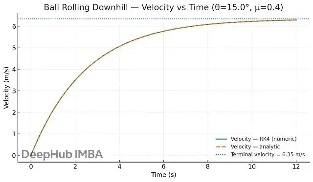

重力把球往下拉，速度快速上升，但摩擦力越來越大，最終達到終端速度。ODE完美地捕捉了這個平滑的過程。

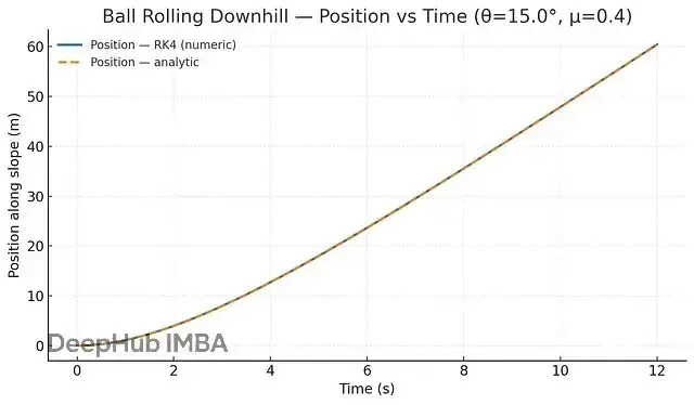
位置的變化也是如此：開始緩慢，然後加速，最後幾乎勻速。這提醒我們，自然界的運動是連續的流，而不是離散的跳躍。

從深度網絡到ODE

傳統深度學習是離散的：

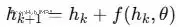
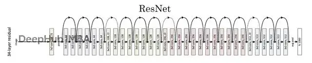
比如説ResNet的每一層都在做同樣事：取當前隱藏狀態，加上一些變換，然後傳遞給下一層。這和數值求解ODE的歐拉方法非常相似——通過小步長逼近連續變化。

或者可以説ResNet其實就是ODE的離散化版本。

更多層應該帶來更強的學習能力。但實際上網絡太深反而性能下降，原因是梯度消失——學習信號在層層傳遞中變得越來越弱。

ResNet的關鍵發現是是引入殘差學習。不要求每層學習完整的變換，而是學習一個"修正項"：

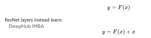
F(x)是殘差，x是跳躍連接傳遞的原始輸入。簡單的説：保留原來的信息，只學習需要調整的部分。

跳躍連接字面上就是把輸入x加到輸出上，這讓梯度能更容易地向後傳播也防止了信息丟失。通過這個技巧，凱明大佬訓練了152層的網絡，ResNet不僅贏了2015年的ImageNet競賽，也成為了現代計算機視覺的基礎框架。

這是一個簡單的ResNet塊實現：

 import torch.nn as nn  

# 定義單個ResNet"塊"  
# 每個塊學習殘差函數F(x)，然後在最後將輸入x加回  
class ResNetBlock(nn.Module):  
    def __init__(self, in_channels, out_channels):  
        super().__init__()  
          
        # 第一個卷積層：  
        # - 應用3x3濾波器從輸入中提取特徵  
        # - padding=1確保輸出大小與輸入相同  
        self.conv1 = nn.Conv2d(in_channels, out_channels, kernel_size=3, padding=1)  
          
        # 非線性：ReLU將非線性模式引入網絡  
        self.relu  = nn.ReLU()  
          
        # 第二個卷積層：  
        # - 另一個3x3濾波器來細化特徵  
        # - 仍然保持空間大小不變  
        self.conv2 = nn.Conv2d(out_channels, out_channels, kernel_size=3, padding=1)  

    def forward(self, x):  
        # 將輸入保存為'殘差'  
        # 這將在稍後通過跳躍連接加回  
        residual = x                       
          
        # 通過第一個卷積 + ReLU激活傳遞輸入  
        out = self.relu(self.conv1(x))  
          
        # 通過第二個卷積傳遞（還沒有激活）  
        out = self.conv2(out)  
          
        # 將原始輸入（殘差）加到輸出上  
        # 這是使ResNet特殊的"跳躍連接"  
        out = out + residual               
          
        # 再次應用ReLU以僅保留正激活  
         return self.relu(out)

關鍵在最後一行：返回的不是out，而是out + residual。這就是ResNet的精髓。

Neural ODE的核心思想

常規深度網絡中，數據要經過固定數量的層。網絡深度必須在訓練前確定——10層、50層還是100層？Neural ODE徹底改變了這個思路。

不再用離散的層，而是讓網絡的隱藏狀態在時間維度上連續演化。不是"通過100層處理輸入"，而是"從初始隱藏狀態開始，讓它按照某個規則連續演化"。

要知道隱藏狀態在某個時刻的樣子，就用ODE求解器，這個算法會問：狀態變化有多快？需要多精確？步長應該多大？

這帶來了一個關鍵特性：自適應深度。標準網絡的深度是固定的，但Neural ODE中求解器自己決定需要多少步。簡單數據用幾步就夠了，複雜數據就多用幾步，網絡在計算過程中自動調整"深度"。

Neural ODE的幾個優勢：

內存效率：不需要存儲所有中間激活，只要起點和終點。

自適應計算：簡單問題少用計算，複雜問題多用計算。

連續建模：天然適合物理、生物、金融等連續變化的系統。

可逆性：對生成模型特別有用。

構建Neural ODE

torchdiffeq

是PyTorch的Neural ODE庫：

 pip install torchdiffeq  
 import torch  
 import torch.nn as nn  
 from torchdiffeq import odeint

定義ODE的動力學函數：

 import torch  
import torch.nn as nn  

class ODEFunc(nn.Module):  
    def __init__(self):  
        super().__init__()  
        # 定義參數化f_theta(h)的神經網絡  
        # 輸入：h（大小為2的狀態向量）  
        # 輸出：dh/dt（h的變化率，也是大小2）  
        self.net = nn.Sequential(  
            nn.Linear(2, 50),   # 層：從2D狀態 -> 50個隱藏單元  
            nn.Tanh(),          # 非線性激活以獲得靈活性  
            nn.Linear(50, 2)    # 層：從50個隱藏單元 -> 2D輸出  
        )  
          
    def forward(self, t, h):  
        """  
        ODE函數的前向傳播。  
        參數：  
            t : 當前時間（標量，odeint需要但這裏未使用）  
            h : 當前狀態（形狀為[batch_size, 2]的張量）  
        返回：  
            dh/dt : h的估計變化率（與h形狀相同）  
        """  
         return self.net(h)

這裏f(h, t, θ)是個小神經網絡，它描述了隱藏狀態如何隨時間變化。

設置初始狀態和時間：

 h0 = torch.tensor([[2., 0.]])   # 起始點
 t = torch.linspace(0, 25, 100)  # 時間步長
 func = ODEFunc()   # 你的神經ODE動力學（dh/dt = f(h)）

求解ODE：

 trajectory = odeint(func, h0, t)  
 print(trajectory.shape)  # (時間, 批次, 特徵)

這樣我們就把神經網絡轉換成了連續系統。

案例研究：捕食者-獵物動力學

這是個經典的生態學問題。雪兔和加拿大猞猁的種羣數量呈現週期性變化：兔子多了，猞猁有足夠食物，數量增加；猞猁多了，兔子被吃得多，數量下降；兔子少了，猞猁沒東西吃，數量也下降；猞猁少了，兔子又開始繁盛...這個循環不斷重複。

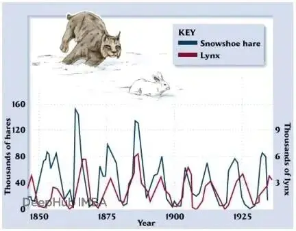
這種動力學天然適合用微分方程建模，Neural ODE可以直接從歷史數據中學習這個系統的演化規律，產生平滑的軌跡，並預測未來的種羣變化。

為什麼捕食者-獵物系統適合用ODE建模？

連續變化：種羣不會突然跳躍，而是隨着動物的出生、死亡平滑變化。

相互依賴：獵物的增長率不只取決於自身繁殖，還取決於捕食者數量。捕食者的生存也依賴獵物的可獲得性。

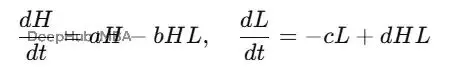
這裏H是兔子，L是猞猁，a是獵物出生率，b是捕食率，c是捕食者死亡率，d是捕食者繁殖率。

反饋循環：更多獵物→捕食者增長→獵物衰落→捕食者餓死→獵物恢復→週期繼續。這些反饋自然形成ODE系統。

預測能力：通過求解方程，我們不僅能描述過去的週期，還能預測或模擬不同條件下的演化。

代碼實現

 !pip -q install torchdiffeq statsmodels  
import math, numpy as np, torch, torch.nn as nn  
import matplotlib.pyplot as plt  
from torchdiffeq import odeint  
from statsmodels.datasets import sunspots  
DEVICE = "cuda" if torch.cuda.is_available() else "cpu"  
torch.manual_seed(1337)  
np.random.seed(1337)  
 print("Device:", DEVICE)

加載哈德遜灣公司的歷史數據（1900-1920年的毛皮貿易記錄）：

# 真實年度毛皮計數（種羣的代理），1900-1920（21年）  
years = np.arange(1900, 1921, dtype=np.int32)  

# 來自經典生態學教科書（四捨五入）  
hares = np.array([30, 47.2, 70.2, 77.4, 36.3, 20.6, 18.1, 21.4, 22.0, 25.4,  
                  27.1, 40.3, 57.0, 76.6, 52.3, 19.5, 11.2,  7.6, 14.6, 16.2, 24.7], dtype=np.float32)  
lynx  = np.array([ 4,  6.1,  9.8, 35.2, 59.4, 41.7, 19.0, 13.0,  8.3,  9.1,  
                  10.8, 12.6, 16.8, 20.6, 18.1,  8.0,  5.3,  3.8,  4.0,  6.5,  8.0], dtype=np.float32)  

assert len(years) == len(hares) == len(lynx)  
N = len(years)  
print(f"Years {years[0]}–{years[-1]} (N={N})")  

# 將數據放入張量並輕度標準化。  
# 種羣是正數且偏斜的；log1p有幫助，然後z-score用於縮放。  
X_raw = np.stack([hares, lynx], axis=1)              # 形狀 (N, 2)  
X_log = np.log1p(X_raw)  
X_mean = X_log.mean(axis=0, keepdims=True)  
X_std  = X_log.std(axis=0, keepdims=True) + 1e-8  
X      = (X_log - X_mean) / X_std                    # 標準化 (N, 2)  

# 時間軸：居中以從0開始，使用年作為連續單位  
t_year = years.astype(np.float32)  
t0 = t_year[0]  
t  = (t_year - t0)                                   # (N,)  
t  = torch.tensor(t, dtype=torch.float32, device=DEVICE)  
Y  = torch.tensor(X, dtype=torch.float32, device=DEVICE)  # (N,2)  

# 訓練/測試分割：擬合80%，預測最後20%  
split = int(0.8 * N)  
t_tr, y_tr = t[:split], Y[:split]  
t_te, y_te = t[split:], Y[split:]  

print("Train points:", len(t_tr), " Test points:", len(t_te))

種羣數據有很大的變化範圍且嚴格為正，所以用log1p穩定尺度，再用z-score標準化便於優化。

定義Neural ODE模型。我們直接建模2D狀態[兔子,猞猁]，ODE右端是個小的MLP，接收當前狀態和時間特徵，輸出狀態的變化率：

    class ODEFunc(nn.Module):  
        """  
        參數化dx/dt = f_theta(x, t)。  
        我們包含簡單的時間特徵（sin/cos）以允許輕微的非平穩性。  
        """  
        def __init__(self, xdim=2, hidden=64, periods=(8.0, 11.0)):  
            super().__init__()  
            self.periods = torch.tensor(periods, dtype=torch.float32)  
            # 輸入：x (2) + 時間特徵 (2 * [#periods](#periods))  
            in_dim = xdim + 2 * len(periods)  
            self.net = nn.Sequential(  
                nn.Linear(in_dim, hidden), nn.Tanh(),  
                nn.Linear(hidden, hidden), nn.Tanh(),  
                nn.Linear(hidden, xdim),  
            )  
            # 温和初始化以避免早期流動爆炸  
            with torch.no_grad():  
                for m in self.net:  
                    if isinstance(m, nn.Linear):  
                        m.weight.mul_(0.1); nn.init.zeros_(m.bias)  

        def _time_feats(self, t_scalar, batch, device):  
            # 構建[sin(2πt/P_k), cos(2πt/P_k)]特徵  
            tt = t_scalar * torch.ones(batch, 1, device=device)  
            feats = []  
            for P in self.periods.to(device):  
                w = 2.0 * math.pi / P  
                feats += [torch.sin(w * tt), torch.cos(w * tt)]  
            return torch.cat(feats, dim=1) if feats else torch.zeros(batch, 0, device=device)  

        def forward(self, t, x):  
            # x: (B, 2) 當前狀態  
            B = x.shape[0]  
            phi_t = self._time_feats(t, B, x.device)  
            return self.net(torch.cat([x, phi_t], dim=1))   # (B,2)  
    class NeuralODE_PredPrey(nn.Module):  
        """  
        從可學習的初始狀態x0在給定時間戳上積分ODE。  
        我們將積分軌跡直接與觀察到的x(t)比較。  
        """  
        def __init__(self, hidden=64, method="dopri5", rtol=1e-4, atol=1e-4, max_num_steps=2000):  
            super().__init__()  
            self.func = ODEFunc(xdim=2, hidden=hidden)  
            # 標準化空間中的可學習初始條件  
            self.x0 = nn.Parameter(torch.zeros(1, 2))  # (1,2)  
            # ODE求解器配置  
            self.method = method  
            self.rtol = rtol  
            self.atol = atol  
            self.max_num_steps = max_num_steps  

        def forward(self, t):  
            """  
            從x0開始在時間t上積分（廣播到batch=1）。  
            返回軌跡(N, 1, 2) -> 我們將壓縮為(N,2)。  
            """  
            opts = {"max_num_steps": self.max_num_steps}  
            x_traj = odeint(self.func, self.x0, t, method=self.method,  
                            rtol=self.rtol, atol=self.atol, options=opts)  
            return x_traj.squeeze(1)   # (N,2)

這裏加入了傅立葉時間特徵（8年和11年週期）來幫助捕捉週期性行為。使用dopri5自適應求解器保持振盪特性。

訓練過程中同時學習ODE動力學和初始狀態，並使用早停機制避免過擬合：

# === 步驟3：訓練與早停 + 最佳檢查點 ===  
import os, json, numpy as np, torch, torch.nn as nn  
import matplotlib.pyplot as plt  

# 模型（與之前相同的超參數；如果你改變了它們請調整）  
model = NeuralODE_PredPrey(hidden=64, method="dopri5", rtol=1e-4, atol=1e-4).to(DEVICE)  
opt    = torch.optim.AdamW(model.parameters(), lr=3e-3, weight_decay=1e-4)  
loss_fn= nn.MSELoss()  

# 訓練配置  
EPOCHS   = 3000          # 上限；如果驗證停止改進我們會提前停止  
PATIENCE = 50            # 等待改進的輪數（你的曲線顯示~50-60最佳）  
BESTPATH = "best_predprey.pt"   # 最佳模型的檢查點路徑  

best_te = float("inf")  
stale   = 0  
hist    = {"epoch": [], "train_mse": [], "test_mse": []}  
best_info = {"epoch": None, "test_mse": None}  

for ep in range(1, EPOCHS + 1):  
    # ---- 在訓練網格上訓練 ----  
    model.train(); opt.zero_grad()  
    yhat_tr   = model(t_tr)                 # (Ntr,2)  
    train_mse = loss_fn(yhat_tr, y_tr)  
    train_mse.backward()  
    torch.nn.utils.clip_grad_norm_(model.parameters(), 1.0)  
    opt.step()  

    # ---- 在測試網格上驗證（評估完整軌跡然後切片） ----  
    model.eval()  
    with torch.no_grad():  
        yhat_all = model(t)                 # (N,2)  
        test_mse = loss_fn(yhat_all[split:], y_te)  

    # ---- 日誌 ----  
    hist["epoch"].append(ep)  
    hist["train_mse"].append(float(train_mse.item()))  
    hist["test_mse"].append(float(test_mse.item()))  

    # ---- 每50輪詳細輸出 ----  
    if ep % 50 == 0:  
        print(f"Epoch {ep:4d} | Train MSE {train_mse.item():.5f} | Test MSE {test_mse.item():.5f}")  

    # ---- 早停邏輯（基於測試MSE） ----  
    if test_mse.item() + 1e-8 < best_te:  
        best_te = test_mse.item()  
        stale   = 0  
        best_info["epoch"]   = ep  
        best_info["test_mse"]= float(best_te)  
        # 保存最佳檢查點（僅權重）  
        torch.save({"model_state": model.state_dict(),  
                    "epoch": ep,  
                    "test_mse": float(best_te)}, BESTPATH)  
    else:  
        stale += 1  
        if stale >= PATIENCE:  
            print(f"⏹️ 在第{ep}輪早停（驗證{PATIENCE}輪無改進）。"  
                  f"最佳輪次 = {best_info['epoch']} 測試MSE = {best_info['test_mse']:.5f}")  
            break  

# ---- 恢復最佳檢查點 ----  
ckpt = torch.load(BESTPATH, map_location=DEVICE)  
model.load_state_dict(ckpt["model_state"])  
print(f"✅ 恢復最佳模型 @ 第{ckpt['epoch']}輪 | 最佳測試MSE = {ckpt['test_mse']:.5f}")  

# ---- 繪製學習曲線與最佳輪次標記 ----  
epochs   = np.array(hist["epoch"], dtype=int)  
train_m  = np.array(hist["train_mse"], dtype=float)  
test_m   = np.array(hist["test_mse"], dtype=float)  
best_ep  = int(best_info["epoch"]) if best_info["epoch"] is not None else int(epochs[np.nanargmin(test_m)])  
best_val = float(best_info["test_mse"]) if best_info["test_mse"] is not None else float(np.nanmin(test_m))  

plt.figure(figsize=(8,4))  
plt.plot(epochs, train_m, label="Train MSE", linewidth=2)  
plt.plot(epochs, test_m,  label="Test MSE",  linewidth=2, linestyle="--")  
plt.axvline(best_ep, color="gray", linestyle=":", label=f"Best Test @ {best_ep} (MSE={best_val:.4f})")  
plt.xlabel("Epoch"); plt.ylabel("MSE (normalized space)")  
plt.title("Learning Curves (Train vs Test) with Early Stopping")  
plt.grid(True, alpha=.3); plt.legend()  
plt.tight_layout(); plt.show()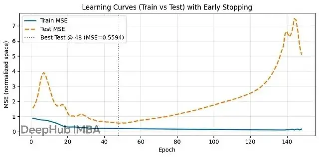

這個學習曲線展示了典型的過擬合過程。前48輪訓練和測試誤差一起下降，測試MSE達到最低值。之後訓練誤差繼續改善，但測試誤差開始上升——模型開始記憶訓練數據的噪聲，而不是學習真正的規律。這就是為什麼我們需要早停機制。

可視化結果時，還需要把標準化的數據轉換回原始單位，這樣更容易理解：

# ===== 步驟4：評估 + 可視化 =====  
import numpy as np, torch, torch.nn.functional as F  
import matplotlib.pyplot as plt  
from pathlib import Path  
from scipy.stats import pearsonr  

# 1) 恢復最佳檢查點（如果尚未恢復）  
ckpt = torch.load(BESTPATH, map_location=DEVICE)  
model.load_state_dict(ckpt["model_state"])  
model.eval()  

# 2) 輔助函數：反標準化回原始毛皮計數  
def denorm(X_norm: torch.Tensor) -> torch.Tensor:  
    X_log = X_norm * torch.tensor(X_std.squeeze(), device=X_norm.device) + torch.tensor(X_mean.squeeze(), device=X_norm.device)  
    return torch.expm1(X_log)  # log1p的逆  

# 3) 在完整時間線（訓練+測試）上預測並分割  
with torch.no_grad():  
    Yhat = model(t)                   # (N,2) 標準化空間  
Y_den    = denorm(Y)                  # (N,2) 原始單位  
Yhat_den = denorm(Yhat)               # (N,2) 原始單位  

# Numpy視圖  
hares_obs, lynx_obs   = Y_den[:,0].cpu().numpy(),   Y_den[:,1].cpu().numpy()  
hares_pred, lynx_pred = Yhat_den[:,0].cpu().numpy(), Yhat_den[:,1].cpu().numpy()  

# 4) 指標（標準化空間）  
def mse(a,b): return float(np.mean((a-b)**2))  
def mae(a,b): return float(np.mean(np.abs(a-b)))  

y_np      = Y.cpu().numpy()  
yhat_np   = Yhat.detach().cpu().numpy()  
y_tr, y_te      = y_np[:split],     y_np[split:]  
yhat_tr, yhat_te= yhat_np[:split], yhat_np[split:]  

mse_tr = mse(y_tr, yhat_tr); mae_tr = mae(y_tr, yhat_tr)  
mse_te = mse(y_te, yhat_te); mae_te = mae(y_te, yhat_te)  
r_te   = pearsonr(y_te.reshape(-1), yhat_te.reshape(-1))[0]  

print(f"Train  MSE={mse_tr:.4f} MAE={mae_tr:.4f}")  
print(f"Test   MSE={mse_te:.4f} MAE={mae_te:.4f}  | Pearson r (test)={r_te:.3f}")  

# 5) 圖表  
split_year = years[split-1]  

# (A) 時間序列疊加：兔子  
plt.figure(figsize=(10,3.6))  
plt.plot(years, hares_obs, 'k-', lw=2, label="Hares (Observed)")  
plt.plot(years, hares_pred, 'b--', lw=2, label="Hares (Neural ODE)")  
plt.axvline(split_year, color='gray', ls='--', alpha=.7, label="Train/Test split")  
plt.xlabel("Year"); plt.ylabel("Pelts (proxy for population)")  
plt.title("Hares: Observed vs Neural ODE")  
plt.grid(alpha=.3); plt.legend(); plt.tight_layout(); plt.show()  

# (B) 時間序列疊加：猞猁  
plt.figure(figsize=(10,3.6))  
plt.plot(years, lynx_obs, 'k-', lw=2, label="Lynx (Observed)")  
plt.plot(years, lynx_pred, 'r--', lw=2, label="Lynx (Neural ODE)")  
plt.axvline(split_year, color='gray', ls='--', alpha=.7)  
plt.xlabel("Year"); plt.ylabel("Pelts (proxy for population)")  
plt.title("Lynx: Observed vs Neural ODE")  
plt.grid(alpha=.3); plt.legend(); plt.tight_layout(); plt.show()  

# (C) 預測放大（僅測試區域）  
plt.figure(figsize=(8,3.6))  
plt.plot(years[split:], hares_obs[split:], 'k-', lw=2, label="Hares (Obs)")  
plt.plot(years[split:], hares_pred[split:], 'b--', lw=2, label="Hares (Pred)")  
plt.plot(years[split:], lynx_obs[split:],  'k-', lw=1.5, alpha=.6, label="Lynx (Obs)")  
plt.plot(years[split:], lynx_pred[split:], 'r--', lw=1.8, label="Lynx (Pred)")  
plt.xlabel("Year"); plt.ylabel("Pelts")  
plt.title("Forecast Region (Test Years)")  
plt.grid(alpha=.3); plt.legend(); plt.tight_layout(); plt.show()  

# (D) 相位肖像：兔子 vs 猞猁  
plt.figure(figsize=(5.6,5.2))  
plt.plot(hares_obs, lynx_obs, 'k.-', label="Observed")  
plt.plot(hares_pred, lynx_pred, 'c.-', label="Neural ODE")  
plt.xlabel("Hares (pelts)"); plt.ylabel("Lynx (pelts)")  
plt.title("Phase Portrait: Predator–Prey Cycle")  
plt.grid(alpha=.3); plt.legend(); plt.tight_layout(); plt.show()  

# (E) 隨時間的殘差（原始單位的絕對誤差）  
abs_err_hares = np.abs(hares_pred - hares_obs)  
abs_err_lynx  = np.abs(lynx_pred  - lynx_obs)  

plt.figure(figsize=(10,3.4))  
plt.plot(years, abs_err_hares, label="|Error| Hares", lw=1.8)  
plt.plot(years, abs_err_lynx,  label="|Error| Lynx",  lw=1.8)  
plt.axvline(split_year, color='gray', ls='--', alpha=.7)  
plt.xlabel("Year"); plt.ylabel("Absolute Error (pelts)")  
plt.title("Prediction Errors over Time")  
plt.grid(alpha=.3); plt.legend(); plt.tight_layout(); plt.show()  

# (F) 觀察 vs 預測散點圖（原始單位）+ R^2  
def r2_score(y_true, y_pred):  
    y_true = np.asarray(y_true); y_pred = np.asarray(y_pred)  
    ss_res = np.sum((y_true - y_pred)**2)  
    ss_tot = np.sum((y_true - y_true.mean())**2) + 1e-12  
    return 1.0 - ss_res/ss_tot  

r2_hares = r2_score(hares_obs[split:], hares_pred[split:])  
r2_lynx  = r2_score(lynx_obs[split:],  lynx_pred[split:])  

plt.figure(figsize=(9,3.6))  
plt.subplot(1,2,1)  
plt.scatter(hares_obs[split:], hares_pred[split:], s=35, alpha=.85)  
plt.plot([hares_obs.min(), hares_obs.max()],  
         [hares_obs.min(), hares_obs.max()], 'k--', lw=1)  
plt.title(f"Hares (Test): R²={r2_hares:.2f}")  
plt.xlabel("Observed"); plt.ylabel("Predicted"); plt.grid(alpha=.3)  

plt.subplot(1,2,2)  
plt.scatter(lynx_obs[split:], lynx_pred[split:], s=35, alpha=.85, color='tab:red')  
plt.plot([lynx_obs.min(), lynx_obs.max()],  
         [lynx_obs.min(), lynx_obs.max()], 'k--', lw=1)  
plt.title(f"Lynx (Test): R²={r2_lynx:.2f}")  
plt.xlabel("Observed"); plt.ylabel("Predicted"); plt.grid(alpha=.3)  

plt.tight_layout(); plt.show()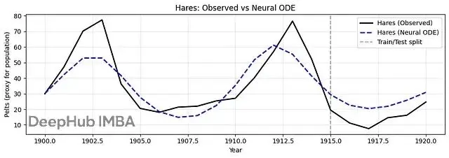

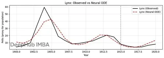
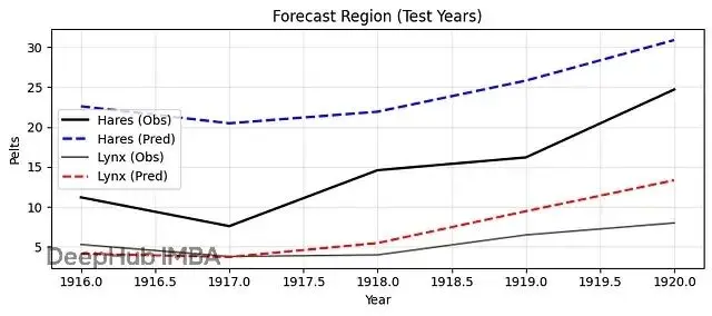
結果顯示Neural ODE成功捕捉了捕食者-獵物系統的週期性動力學。模型學會了兔子和猞猁種羣的相互依賴關係，能夠產生平滑的預測軌跡。

如果擬合效果不夠好，可以嘗試：延長訓練時間（

EPOCHS=5000

），增加網絡容量（

hidden=96

），或者調低學習率（

lr=2e-3

）。

總結

通過一個實際案例我們看到了Neural ODE技術的強大潛力。它不僅是數學上的優雅理論，更是解決實際問題的有力工具。

Neural ODE的核心價值在於連續性思維：世界本質上是連續的，而傳統深度學習的離散化可能丟失重要信息。通過引入微分方程，我們能夠更自然地建模連續過程，處理不規律的時間序列數據，獲得更好的數值穩定性，並實現更精確的時間建模。

當然Neural ODE也並非萬能。它的計算成本較高，對初值敏感，調參也相對複雜。但隨着硬件算力提升和算法優化，這些問題正在逐步解決。

正如物理學家費曼所説："我們需要的不僅是計算能力，更是對自然規律的深刻理解。"Neural ODE正是這種理解與計算的完美結合。

https://avoid.overfit.cn/post/af8511a953524409b9f41fd27d5958b7

作者：Rayan Yassminh