

目前來看Google 是唯一一家在 AI 價值鏈上實現端到端垂直整合的公司。從基礎模型 (Gemini)、應用層 (ImageFX, Search with Gemini, NotebookLM),到雲架構 (Google Cloud, Vertex AI) 以及硬件 (TPUs),幾乎全都有所佈局。
長期以來Google 一直在通過提升自身能力來減少對 NVIDIA GPU 的依賴。這種技術積累逐漸演變成了現在的 JAX AI 棧。

更有意思的是這套技術棧現在不僅 Google 自己用,Anthropic、xAI 甚至 Apple 這些頭部 LLM 提供商也都在用
所以我們就很有必要這就很有必要深入聊聊這套技術棧了。
什麼是 JAX AI 棧?
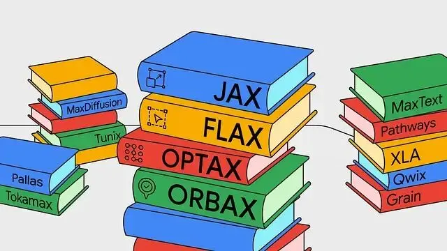
簡單來説,JAX AI 棧是一套面向超大規模機器學習的端到端開源平台。
核心組件主要由以下四個部分構成:
1、JAX
Google 和 NVIDIA 聯合開發的 Python 高性能數值計算庫。
接口設計極其類似 NumPy,但區別在於它能自動、高效地在 CPU、GPU 或 TPU 上運行,無論是本地還是分佈式環境。
底層的技術在於 XLA (Accelerated Linear Algebra) 編譯器,它能把 JAX 代碼轉譯成針對不同硬件深度優化的機器碼。對比之下NumPy 的操作默認只能在 CPU 上跑,效率天差地別。
2、Flax
基於 JAX 的神經網絡訓練庫。Flax 的核心現在是 NNX (Neural Networks for JAX)。這是一個簡化版的 API,讓創建、調試和分析 JAX 神經網絡變得更直觀。
之前有個 Flax Linen,是那種無狀態、函數式風格的 API。而 NNX 作為繼任者,引入了面向對象和有狀態的特性,對於習慣了 PyTorch 的開發者來説,構建和調試 JAX 模型會順手很多。
3、Optax
JAX 生態裏的梯度處理和優化庫。
它的優勢在於靈活性,幾行代碼就能把標準優化器和複雜的技巧(比如梯度裁剪、梯度累積)鏈式組合起來。
4. Orbax
專門處理 Checkpoint 的庫,用於保存和恢復大規模訓練任務。
支持異步分佈式檢查點,這在大模型訓練裏至關重要——萬一硬件掛了,能從斷點恢復,不至於讓昂貴的算力打了水漂。
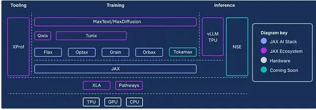
下面這張圖展示了完整棧的架構,除了上面這四個核心,還有很多其他組件,建議細看。
實戰:用 JAX 訓練神經網絡
JAX 之所以在 GPU 和 TPU 上能跑贏 PyTorch,主要歸功於即時 (JIT) 優化和 XLA 的後端編譯效率。
我們直接上手用 JAX 擼一個簡單的神經網絡,搞個手寫數字識別,看看這套棧在實際工作流裏到底怎麼用。
1、環境配置
JAX AI 棧現在整合成了一個 metapackage,安裝很簡單。然後我們還需要
sklearn(加載數據)和
matplotlib(畫圖)。
!uv pip install jax-ai-stack sklearn matplotlib2、加載數據
直接用 sklearn 加載 UCI ML 手寫數字數據集。
 fromsklearn.datasetsimportload_digits

 # Load dataset
 digits=load_digits()
數據是
8 x 8的像素化手寫數字圖像(0 到 9)及其對應的標籤。
 print(f"Number of samples × features: {digits.data.shape}")
 print(f"Number of labels: {digits.target.shape}")

 """
 Number of samples × features: (1797, 64)
 Number of labels: (1797,)
 """
3、 數據可視化
先看看數據長什麼樣,挑 100 張圖畫出來。
 import matplotlib.pyplot as plt

fig, axes = plt.subplots(10, 10, figsize=(6, 6),
                         subplot_kw={'xticks':[], 'yticks':[]},
                         gridspec_kw=dict(hspace=0.1, wspace=0.1))

for i, ax in enumerate(axes.flat):
    ax.imshow(digits.images[i], cmap='binary', interpolation='gaussian')
     ax.text(0.05, 0.05, str(digits.target[i]), transform=ax.transAxes, color='green')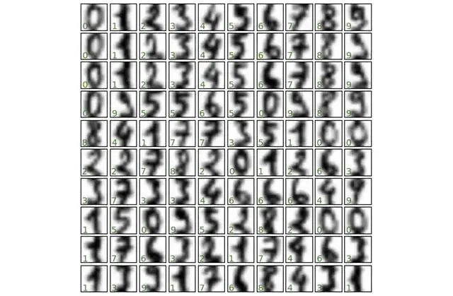
4、 數據集切分
常規操作,把數據切成訓練集和測試集。
 from sklearn.model_selection import train_test_split

 # Create dataset splits
 splits = train_test_split(digits.images, digits.target, random_state=0)
5、轉為 JAX 數組
這一步很關鍵,輸入到模型之前,需要用 JAX Numpy 把數據轉成 JAX 數組格式。
 import jax.numpy as jnp

 # Convert splits to JAX arrays
 images_train, images_test, label_train, label_test = map(jnp.asarray, splits)
看一眼數據維度:
 print(f"Training images shape: {images_train.shape}")
print(f"Training labels shape: {label_train.shape}")
print(f"Test images shape: {images_test.shape}")
print(f"Test labels shape: {label_test.shape}")

"""
Training images shape: (1347, 8, 8)
Training labels shape: (1347,)
Test images shape: (450, 8, 8)
Test labels shape: (450,)
 """
6、用 Flax 構建網絡
用 Flax NNX 搭建一個帶 SELU 激活函數的簡單前饋網絡。習慣寫 PyTorch 的朋友會發現,這語法看着非常眼熟。
 from flax import nnx

class DigitClassifier(nnx.Module):
  def __init__(self, n_features, n_hidden, n_targets, rngs):
    self.n_features = n_features
    self.layer_1 = nnx.Linear(n_features, n_hidden, rngs = rngs)
    self.layer_2 = nnx.Linear(n_hidden, n_hidden, rngs = rngs)
    self.layer_3 = nnx.Linear(n_hidden, n_targets, rngs = rngs)

  def __call__(self, x):
    x = x.reshape(x.shape[0], self.n_features) [#Flatten](#Flatten) images
    x = nnx.selu(self.layer_1(x))
    x = nnx.selu(self.layer_2(x))
    x = self.layer_3(x)
     return x
7、實例化模型
JAX 處理隨機數的方式比較特別。這裏用
nnx.Rngs(0)初始化一個種子為 0 的隨機數生成器 (RNG) 對象。這個對象負責管理網絡操作裏的所有隨機性,比如參數初始化和 Dropout。
注意,這和 PyTorch 直接設全局種子
torch.manual_seed(seed)的邏輯不一樣。
 # Initialize random number generator
 rngs = nnx.Rngs(0)

 # Create instance of the classifier
 model = DigitClassifier(n_features=64, n_hidden=128, n_targets=10, rngs = rngs)
8、定義優化器與訓練步驟
用 Optax 定義優化器和損失函數。
 import jax
import optax

# SGD optimizer with learning rate 0.05
optimizer = nnx.ModelAndOptimizer(
    model, optax.sgd(learning_rate=0.05))

# Loss function
def loss_fn(model, data, labels):
    # Forward pass
    logits = model(data)

    # Compute mean cross-entropy loss
    loss = optax.softmax_cross_entropy_with_integer_labels(
    logits=logits, labels=labels).mean()

    return loss, logits

# Single training step with automatic differentiation and optimization
@nnx.jit  # JIT compile for faster execution
def training_step(model, optimizer, data, labels):
    loss_gradient = nnx.grad(loss_fn, has_aux=True)  # 'has_aux=True' allows returning auxiliary outputs (logits)
    grads, logits = loss_gradient(model, data, labels)  # Forward + backward pass
     optimizer.update(grads)  # Update model parameters using computed gradients
代碼裏用到了兩個核心變換,這是 JAX 高效的秘訣:
jax.jit:即時編譯,把訓練函數扔給 XLA 編譯器,重複執行速度極快。
jax.grad:利用自動微分計算梯度。
Flax NNX 把它倆封裝成了裝飾器
nnx.jit和
nnx.grad,用起來更方便。
9、訓練循環
跑 500 epoch,每 100 輪顯示 Loss。
 num_epochs=500
print_every=100

forepochinrange(num_epochs+1):
  # Training step
  training_step(model, optimizer, images_train, label_train)

  # Evaluate and print metrics periodically
  ifepoch%print_every==0:
    train_loss, _=loss_fn(model, images_train, label_train)
    test_loss, _=loss_fn(model, images_test, label_test)
    print(f"Epoch {epoch:3d} | Train Loss: {train_loss:.4f} | Test Loss: {test_loss:.4f}")

"""
Epoch   0 | Train Loss: 0.0044 | Test Loss: 0.1063
Epoch 100 | Train Loss: 0.0035 | Test Loss: 0.1057
Epoch 200 | Train Loss: 0.0029 | Test Loss: 0.1054
Epoch 300 | Train Loss: 0.0024 | Test Loss: 0.1052
Epoch 400 | Train Loss: 0.0021 | Test Loss: 0.1051
Epoch 500 | Train Loss: 0.0019 | Test Loss: 0.1050
 """
10. 效果評估
最後看看在測試集上的表現。
 # Evaluate model accuracy on test set
logits = model(images_test)

predictions = logits.argmax(axis=1)

correct = jnp.sum(predictions == label_test)

total = len(label_test)

accuracy = correct / total

print(f"Test Accuracy: {correct}/{total} correct ({accuracy:.2%})")
 # Test Accuracy: 437/450 correct (97.11%)
97% 的準確率,對於這麼簡單的網絡來説相當不錯了。
最後把預測結果可視化一下,綠色是對的,紅色是錯的。
 fig, axes = plt.subplots(10, 10, figsize=(6, 6),
                         subplot_kw={'xticks':[], 'yticks':[]},
                         gridspec_kw=dict(hspace=0.1, wspace=0.1))

for i, ax in enumerate(axes.flat):
    ax.imshow(images_test[i], cmap='binary', interpolation='gaussian')
    color = 'green' if label_pred[i] == label_test[i] else 'red'
     ax.text(0.05, 0.05, str(label_pred[i]), transform=ax.transAxes, color=color)
到這裏,你就已經在 JAX 生態裏跑通了第一個神經網絡。JAX 的門檻其實沒那麼高,但它帶來的性能收益,特別是在大規模訓練場景下,絕對值得投入時間去學。
https://avoid.overfit.cn/post/5279caa8ac7f4b1dbe34d90628a58672
作者:Dr. Ashish Bamania